Note
-
Download Jupyter notebook:
https://docs.doubleml.org/stable/examples/did/py_panel_data_example.ipynb.
Python: Real-Data Example for Multi-Period Difference-in-Differences#
In this example, we replicate a real-data demo notebook from the did-R-package in order to illustrate the use of DoubleML for multi-period difference-in-differences (DiD) models.
The notebook requires the following packages:
[1]:
import pyreadr
import pandas as pd
import numpy as np

from sklearn.linear_model import LinearRegression, LogisticRegression
from sklearn.dummy import DummyRegressor, DummyClassifier
from sklearn.linear_model import LassoCV, LogisticRegressionCV

from doubleml.data import DoubleMLPanelData
from doubleml.did import DoubleMLDIDMulti
Causal Research Question#
Callaway and Sant’Anna (2021) study the causal effect of raising the minimum wage on teen employment in the US using county data over a period from 2001 to 2007. A county is defined as treated if the minimum wage in that county is above the federal minimum wage. We focus on a preprocessed balanced panel data set as provided by the did-R-package. The corresponding documentation for the mpdta
data is available from the did package website. We use this data solely as a demonstration example to help readers understand differences in the DoubleML and did packages. An analogous notebook using the same data is available from the did documentation.
We follow the original notebook and provide results under identification based on unconditional and conditional parallel trends. For the Double Machine Learning (DML) Difference-in-Differences estimator, we demonstrate two different specifications, one based on linear and logistic regression and one based on their \(\ell_1\) penalized variants Lasso and logistic regression with cross-validated penalty choice. The results for the former are expected to be very similar to those in the did data example. Minor differences might arise due to the use of sample-splitting in the DML estimation.
Data#
We will download and read a preprocessed data file as provided by the did-R-package.
[2]:
# download file from did package for R
url = "https://github.com/bcallaway11/did/raw/refs/heads/master/data/mpdta.rda"
pyreadr.download_file(url, "mpdta.rda")

mpdta = pyreadr.read_r("mpdta.rda")["mpdta"]
mpdta.head()
[2]:
| year | countyreal | lpop | lemp | first.treat | treat | |
|---|---|---|---|---|---|---|
| 0 | 2003 | 8001.0 | 5.896761 | 8.461469 | 2007.0 | 1.0 |
| 1 | 2004 | 8001.0 | 5.896761 | 8.336870 | 2007.0 | 1.0 |
| 2 | 2005 | 8001.0 | 5.896761 | 8.340217 | 2007.0 | 1.0 |
| 3 | 2006 | 8001.0 | 5.896761 | 8.378161 | 2007.0 | 1.0 |
| 4 | 2007 | 8001.0 | 5.896761 | 8.487352 | 2007.0 | 1.0 |
To work with DoubleML, we initialize a DoubleMLPanelData object. The input data has to satisfy some requirements, i.e., it should be in a long format with every row containing the information of one unit at one time period. Moreover, the data should contain a column on the unit identifier and a column on the time period. The requirements are virtually identical to those of the
did-R-package, as listed in their data example. In line with the naming conventions of DoubleML, the treatment group indicator is passed to DoubleMLPanelData by the d_cols argument. To flexibly handle different formats for handling time periods, the time variable t_col can handle float,
int and datetime formats. More information are available in the user guide. To indicate never treated units, we set their value for the treatment group variable to np.inf.
Now, we can initialize the DoubleMLPanelData object, specifying
y_col: the outcomed_cols: the group variable indicating the first treated period for each unitid_col: the unique identification column for each unitt_col: the time columnx_cols: the additional pre-treatment controls
[3]:
# Set values for treatment group indicator for never-treated to np.inf
mpdta.loc[mpdta['first.treat'] == 0, 'first.treat'] = np.inf

dml_data = DoubleMLPanelData(
    data=mpdta,
    y_col="lemp",
    d_cols="first.treat",
    id_col="countyreal",
    t_col="year",
    x_cols=['lpop']
)
print(dml_data)
================== DoubleMLPanelData Object ==================

------------------ Data summary      ------------------
Outcome variable: lemp
Treatment variable(s): ['first.treat']
Covariates: ['lpop']
Instrument variable(s): None
Time variable: year
Id variable: countyreal
Static panel data: False
No. Unique Ids: 500
No. Observations: 2500
------------------ DataFrame info    ------------------
<class 'pandas.DataFrame'>
RangeIndex: 2500 entries, 0 to 2499
Columns: 6 entries, year to treat
dtypes: float64(5), int32(1)
memory usage: 107.6 KB
Note that we specified a pre-treatment confounding variable lpop through the x_cols argument. To consider cases under unconditional parallel trends, we can use dummy learners to ignore the pre-treatment confounding variable. This is illustrated below.
ATT Estimation: Unconditional Parallel Trends#
We start with identification under the unconditional parallel trends assumption. To do so, initialize a DoubleMLDIDMulti object (see model documentation), which takes the previously initialized DoubleMLPanelData object as input. We use scikit-learn’s DummyRegressor (documentation here) and
DummyClassifier (documentation here) to ignore the pre-treatment confounding variable. At this stage, we can also pass further options, for example specifying the number of folds and repetitions used for cross-fitting.
When calling the fit() method, the model estimates standard combinations of \(ATT(g,t)\) parameters, which corresponds to the defaults in the did-R-package. These combinations can also be customized through the gt_combinations argument, see the user guide.
[4]:
dml_obj = DoubleMLDIDMulti(
    obj_dml_data=dml_data,
    ml_g=DummyRegressor(),
    ml_m=DummyClassifier(),
    control_group="never_treated",
    n_folds=10
)

dml_obj.fit()
print(dml_obj.summary.round(4))
                         coef  std err       t   P>|t|   2.5 %  97.5 %
ATT(2004.0,2003,2004) -0.0105   0.0232 -0.4527  0.6507 -0.0560  0.0350
ATT(2004.0,2003,2005) -0.0704   0.0313 -2.2523  0.0243 -0.1316 -0.0091
ATT(2004.0,2003,2006) -0.1372   0.0364 -3.7721  0.0002 -0.2086 -0.0659
ATT(2004.0,2003,2007) -0.1009   0.0345 -2.9209  0.0035 -0.1686 -0.0332
ATT(2006.0,2003,2004)  0.0065   0.0233  0.2797  0.7797 -0.0392  0.0522
ATT(2006.0,2004,2005) -0.0027   0.0196 -0.1395  0.8890 -0.0412  0.0357
ATT(2006.0,2005,2006) -0.0046   0.0178 -0.2603  0.7946 -0.0395  0.0302
ATT(2006.0,2005,2007) -0.0413   0.0206 -2.0072  0.0447 -0.0816 -0.0010
ATT(2007.0,2003,2004)  0.0306   0.0151  2.0311  0.0422  0.0011  0.0601
ATT(2007.0,2004,2005) -0.0027   0.0164 -0.1650  0.8689 -0.0349  0.0295
ATT(2007.0,2005,2006) -0.0312   0.0179 -1.7453  0.0809 -0.0663  0.0038
ATT(2007.0,2006,2007) -0.0261   0.0167 -1.5642  0.1178 -0.0587  0.0066
The summary displays estimates of the \(ATT(g,t_\text{eval})\) effects for different combinations of \((g,t_\text{eval})\) via \(\widehat{ATT}(\mathrm{g},t_\text{pre},t_\text{eval})\), where
\(\mathrm{g}\) specifies the group
\(t_\text{pre}\) specifies the corresponding pre-treatment period
\(t_\text{eval}\) specifies the evaluation period
This corresponds to the estimates given in att_gt function in the did-R-package, where the standard choice is \(t_\text{pre} = \min(\mathrm{g}, t_\text{eval}) - 1\) (without anticipation).
Remark that this includes pre-tests effects if \(\mathrm{g} > t_{eval}\), e.g. \(ATT(2007,2005)\).
As usual for the DoubleML-package, you can obtain joint confidence intervals via bootstrap.
[5]:
level = 0.95

ci = dml_obj.confint(level=level)
dml_obj.bootstrap(n_rep_boot=5000)
ci_joint = dml_obj.confint(level=level, joint=True)
print(ci_joint)
                          2.5 %    97.5 %
ATT(2004.0,2003,2004) -0.075355  0.054342
ATT(2004.0,2003,2005) -0.157725  0.016944
ATT(2004.0,2003,2006) -0.238924 -0.035569
ATT(2004.0,2003,2007) -0.197384 -0.004364
ATT(2006.0,2003,2004) -0.058639  0.071681
ATT(2006.0,2004,2005) -0.057512  0.052042
ATT(2006.0,2005,2006) -0.054329  0.045070
ATT(2006.0,2005,2007) -0.098743  0.016190
ATT(2007.0,2003,2004) -0.011500  0.072695
ATT(2007.0,2004,2005) -0.048605  0.043184
ATT(2007.0,2005,2006) -0.081179  0.018762
ATT(2007.0,2006,2007) -0.072628  0.020501
A visualization of the effects can be obtained via the plot_effects() method.
Remark that the plot used joint confidence intervals per default.
[6]:
fig, ax = dml_obj.plot_effects()
Effect Aggregation#
As the did-R-package, the \(ATT\)’s can be aggregated to summarize multiple effects. For details on different aggregations and details on their interpretations see Callaway and Sant’Anna(2021).
The aggregations are implemented via the aggregate() method. We follow the structure of the did package notebook and start with an aggregation relative to the treatment timing.
Event Study Aggregation#
We can aggregate the \(ATT\)s relative to the treatment timing. This is done by setting aggregation="eventstudy" in the aggregate() method. aggregation="eventstudy" aggregates \(\widehat{ATT}(\mathrm{g},t_\text{pre},t_\text{eval})\) based on exposure time \(e = t_\text{eval} - \mathrm{g}\) (respecting group size).
[7]:
# rerun bootstrap for valid simultaneous inference (as values are not saved)
dml_obj.bootstrap(n_rep_boot=5000)
aggregated_eventstudy = dml_obj.aggregate("eventstudy")
# run bootstrap to obtain simultaneous confidence intervals
aggregated_eventstudy.aggregated_frameworks.bootstrap()
print(aggregated_eventstudy)
fig, ax = aggregated_eventstudy.plot_effects()
================== DoubleMLDIDAggregation Object ==================
 Event Study Aggregation

------------------ Overall Aggregated Effects ------------------
     coef  std err         t    P>|t|    2.5 %    97.5 %
-0.077262 0.020025 -3.858309 0.000114 -0.11651 -0.038014
------------------ Aggregated Effects         ------------------
          coef   std err         t     P>|t|     2.5 %    97.5 %
-3.0  0.030598  0.015064  2.031130  0.042242  0.001072  0.060124
-2.0 -0.000551  0.013303 -0.041405  0.966973 -0.026625  0.025523
-1.0 -0.024548  0.014213 -1.727112  0.084147 -0.052405  0.003310
0.0  -0.019946  0.011813 -1.688519  0.091312 -0.043098  0.003206
1.0  -0.050981  0.017029 -2.993762  0.002756 -0.084357 -0.017605
2.0  -0.137247  0.036385 -3.772076  0.000162 -0.208560 -0.065934
3.0  -0.100874  0.034536 -2.920864  0.003491 -0.168563 -0.033185
------------------ Additional Information     ------------------
Score function: observational
Control group: never_treated
Anticipation periods: 0
Alternatively, the \(ATT\) could also be aggregated according to (calendar) time periods or treatment groups, see the user guide.
Aggregation Details#
The DoubleMLDIDAggregation objects include several DoubleMLFrameworks which support methods like bootstrap() or confint(). Further, the weights can be accessed via the properties
overall_aggregation_weights: weights for the overall aggregationaggregation_weights: weights for the aggregation
To clarify, e.g. for the eventstudy aggregation
If one would like to consider how the aggregated effect with \(e=0\) is computed, one would have to look at the third set of weights within the aggregation_weights property
[8]:
aggregated_eventstudy.aggregation_weights[2]
[8]:
array([0.        , 0.        , 0.        , 0.        , 0.        ,
       0.23391813, 0.        , 0.        , 0.        , 0.        ,
       0.76608187, 0.        ])
ATT Estimation: Conditional Parallel Trends#
We briefly demonstrate how to use the DoubleMLDIDMulti model with conditional parallel trends. As the rationale behind DML is to flexibly model nuisance components as prediction problems, the DML DiD estimator includes pre-treatment covariates by default. In DiD, the nuisance components are the outcome regression and the propensity score estimation for the treatment group variable. This is why we had to enforce dummy learners in the unconditional parallel trends case to ignore the
pre-treatment covariates. Now, we can replicate the classical doubly robust DiD estimator as of Callaway and Sant’Anna(2021) by using linear and logistic regression for the nuisance components. This is done by setting ml_g to LinearRegression() and ml_m to LogisticRegression(). Similarly, we can also choose other learners, for example by setting ml_g and ml_m to LassoCV() and LogisticRegressionCV(). We present
the results for the ATTs and their event-study aggregation in the corresponding effect plots.
Please note that the example is meant to illustrate the usage of the DoubleMLDIDMulti model in combination with ML learners. In real-data applicatoins, careful choice and empirical evaluation of the learners are required. Default measures for the prediction of the nuisance components are printed in the model summary, as briefly illustrated below.
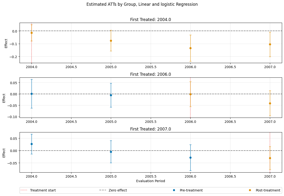
[9]:
dml_obj_linear_logistic = DoubleMLDIDMulti(
    obj_dml_data=dml_data,
    ml_g=LinearRegression(),
    ml_m=LogisticRegression(penalty=None),
    control_group="never_treated",
    n_folds=10
)

dml_obj_linear_logistic.fit()
dml_obj_linear_logistic.bootstrap(n_rep_boot=5000)
dml_obj_linear_logistic.plot_effects(title="Estimated ATTs by Group, Linear and logistic Regression")
[9]:
(<Figure size 1200x800 with 4 Axes>,
 [<Axes: title={'center': 'First Treated: 2004.0'}, ylabel='Effect'>,
  <Axes: title={'center': 'First Treated: 2006.0'}, ylabel='Effect'>,
  <Axes: title={'center': 'First Treated: 2007.0'}, xlabel='Evaluation Period', ylabel='Effect'>])
We briefly look at the model summary, which includes some standard diagnostics for the prediction of the nuisance components.
[10]:
print(dml_obj_linear_logistic)
================== DoubleMLDIDMulti Object ==================

------------------ Data summary      ------------------
Outcome variable: lemp
Treatment variable(s): ['first.treat']
Covariates: ['lpop']
Instrument variable(s): None
Time variable: year
Id variable: countyreal
Static panel data: False
No. Unique Ids: 500
No. Observations: 2500
------------------ Score & algorithm ------------------
Score function: observational
Control group: never_treated
Anticipation periods: 0

------------------ Machine learner   ------------------
Learner ml_g: LinearRegression()
Learner ml_m: LogisticRegression(penalty=None)
Out-of-sample Performance:
Regression:
Learner ml_g0 RMSE: [[0.1719432  0.18246495 0.26051185 0.25982314 0.17301667 0.15169288
  0.20135638 0.20640346 0.17246071 0.15166183 0.20191979 0.164085  ]]
Learner ml_g1 RMSE: [[0.10024991 0.12545934 0.13976841 0.149942   0.14098636 0.11232648
  0.08693238 0.11257581 0.13588417 0.16357232 0.15953874 0.16127052]]
Classification:
Learner ml_m Log Loss: [[0.22998326 0.23122742 0.23233298 0.22988976 0.34996961 0.34790822
  0.34902252 0.35003539 0.60691809 0.6061762  0.6062548  0.60712282]]

------------------ Resampling        ------------------
No. folds: 10
No. repeated sample splits: 1

------------------ Fit summary       ------------------
                           coef   std err         t     P>|t|     2.5 %  \
ATT(2004.0,2003,2004) -0.014495  0.022083 -0.656373  0.511584 -0.057777
ATT(2004.0,2003,2005) -0.075583  0.028329 -2.668028  0.007630 -0.131108
ATT(2004.0,2003,2006) -0.133963  0.035599 -3.763160  0.000168 -0.203735
ATT(2004.0,2003,2007) -0.105078  0.033485 -3.138103  0.001700 -0.170706
ATT(2006.0,2003,2004)  0.000632  0.022177  0.028500  0.977264 -0.042834
ATT(2006.0,2004,2005) -0.005773  0.018314 -0.315233  0.752585 -0.041668
ATT(2006.0,2005,2006) -0.001071  0.019272 -0.055594  0.955666 -0.038843
ATT(2006.0,2005,2007) -0.041319  0.019335 -2.137016  0.032597 -0.079215
ATT(2007.0,2003,2004)  0.026542  0.014166  1.873605  0.060985 -0.001223
ATT(2007.0,2004,2005) -0.004510  0.015755 -0.286259  0.774679 -0.035388
ATT(2007.0,2005,2006) -0.028309  0.018427 -1.536257  0.124475 -0.064426
ATT(2007.0,2006,2007) -0.030379  0.016356 -1.857309  0.063267 -0.062436

                         97.5 %
ATT(2004.0,2003,2004)  0.028788
ATT(2004.0,2003,2005) -0.020059
ATT(2004.0,2003,2006) -0.064191
ATT(2004.0,2003,2007) -0.039449
ATT(2006.0,2003,2004)  0.044098
ATT(2006.0,2004,2005)  0.030122
ATT(2006.0,2005,2006)  0.036700
ATT(2006.0,2005,2007) -0.003423
ATT(2007.0,2003,2004)  0.054307
ATT(2007.0,2004,2005)  0.026369
ATT(2007.0,2005,2006)  0.007808
ATT(2007.0,2006,2007)  0.001679
[11]:
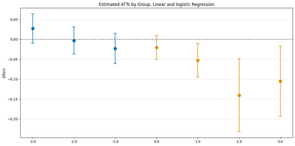
es_linear_logistic = dml_obj_linear_logistic.aggregate("eventstudy")
es_linear_logistic.aggregated_frameworks.bootstrap()
es_linear_logistic.plot_effects(title="Estimated ATTs by Group, Linear and logistic Regression")
[11]:
(<Figure size 1200x600 with 1 Axes>,
 <Axes: title={'center': 'Estimated ATTs by Group, Linear and logistic Regression'}, ylabel='Effect'>)
[12]:
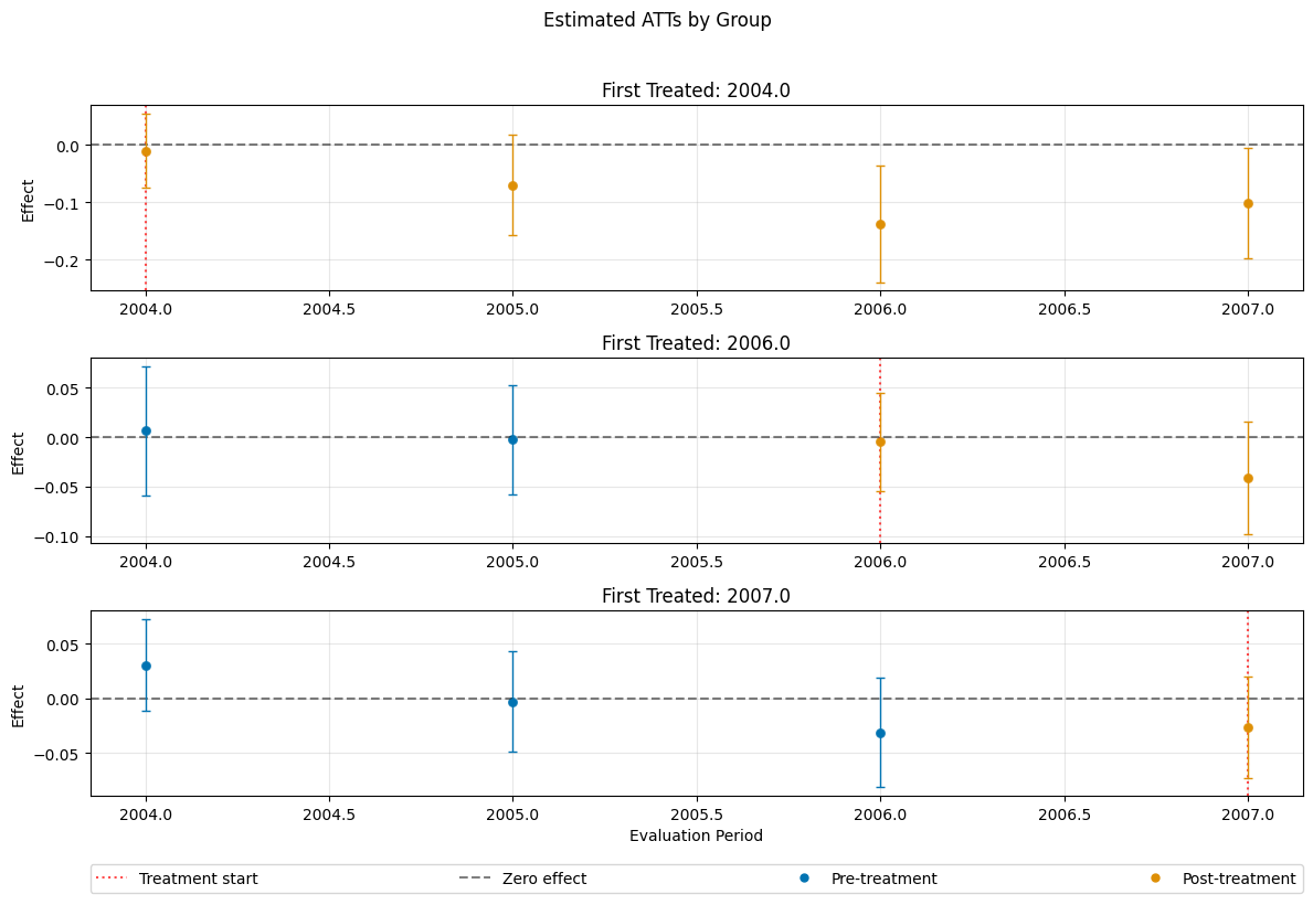
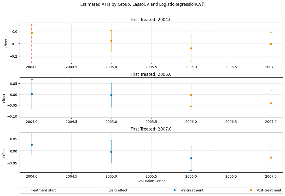
dml_obj_lasso = DoubleMLDIDMulti(
    obj_dml_data=dml_data,
    ml_g=LassoCV(),
    ml_m=LogisticRegressionCV(),
    control_group="never_treated",
    n_folds=10
)

dml_obj_lasso.fit()
dml_obj_lasso.bootstrap(n_rep_boot=5000)
dml_obj_lasso.plot_effects(title="Estimated ATTs by Group, LassoCV and LogisticRegressionCV()")
[12]:
(<Figure size 1200x800 with 4 Axes>,
 [<Axes: title={'center': 'First Treated: 2004.0'}, ylabel='Effect'>,
  <Axes: title={'center': 'First Treated: 2006.0'}, ylabel='Effect'>,
  <Axes: title={'center': 'First Treated: 2007.0'}, xlabel='Evaluation Period', ylabel='Effect'>])
[13]:
# Model summary
print(dml_obj_lasso)
================== DoubleMLDIDMulti Object ==================

------------------ Data summary      ------------------
Outcome variable: lemp
Treatment variable(s): ['first.treat']
Covariates: ['lpop']
Instrument variable(s): None
Time variable: year
Id variable: countyreal
Static panel data: False
No. Unique Ids: 500
No. Observations: 2500
------------------ Score & algorithm ------------------
Score function: observational
Control group: never_treated
Anticipation periods: 0

------------------ Machine learner   ------------------
Learner ml_g: LassoCV()
Learner ml_m: LogisticRegressionCV()
Out-of-sample Performance:
Regression:
Learner ml_g0 RMSE: [[0.1730221  0.18161117 0.25947955 0.25938247 0.17243026 0.15194491
  0.20094004 0.2053522  0.17495733 0.15236128 0.20082045 0.1642811 ]]
Learner ml_g1 RMSE: [[0.09799983 0.13085782 0.13879791 0.14964961 0.1411192  0.11919283
  0.08741588 0.10713135 0.13215504 0.1625061  0.15963555 0.15896281]]
Classification:
Learner ml_m Log Loss: [[0.22913691 0.22913385 0.22913626 0.22913505 0.35596598 0.35596545
  0.35596757 0.35597139 0.60883756 0.60885249 0.60884912 0.60883852]]

------------------ Resampling        ------------------
No. folds: 10
No. repeated sample splits: 1

------------------ Fit summary       ------------------
                           coef   std err         t     P>|t|     2.5 %  \
ATT(2004.0,2003,2004) -0.012407  0.022434 -0.553037  0.580238 -0.056378
ATT(2004.0,2003,2005) -0.076869  0.028893 -2.660498  0.007803 -0.133498
ATT(2004.0,2003,2006) -0.137755  0.035587 -3.870899  0.000108 -0.207506
ATT(2004.0,2003,2007) -0.103678  0.033322 -3.111401  0.001862 -0.168988
ATT(2006.0,2003,2004)  0.000866  0.023612  0.036692  0.970731 -0.045413
ATT(2006.0,2004,2005) -0.003946  0.019365 -0.203749  0.838550 -0.041901
ATT(2006.0,2005,2006) -0.004357  0.017933 -0.242982  0.808020 -0.039505
ATT(2006.0,2005,2007) -0.041231  0.020177 -2.043463  0.041007 -0.080777
ATT(2007.0,2003,2004)  0.026447  0.015322  1.726080  0.084333 -0.003584
ATT(2007.0,2004,2005) -0.003903  0.016467 -0.236995  0.812661 -0.036177
ATT(2007.0,2005,2006) -0.030882  0.017916 -1.723700  0.084762 -0.065997
ATT(2007.0,2006,2007) -0.027356  0.016745 -1.633716  0.102319 -0.060175

                         97.5 %
ATT(2004.0,2003,2004)  0.031564
ATT(2004.0,2003,2005) -0.020240
ATT(2004.0,2003,2006) -0.068005
ATT(2004.0,2003,2007) -0.038368
ATT(2006.0,2003,2004)  0.047146
ATT(2006.0,2004,2005)  0.034009
ATT(2006.0,2005,2006)  0.030790
ATT(2006.0,2005,2007) -0.001685
ATT(2007.0,2003,2004)  0.056477
ATT(2007.0,2004,2005)  0.028372
ATT(2007.0,2005,2006)  0.004233
ATT(2007.0,2006,2007)  0.005463
[14]:
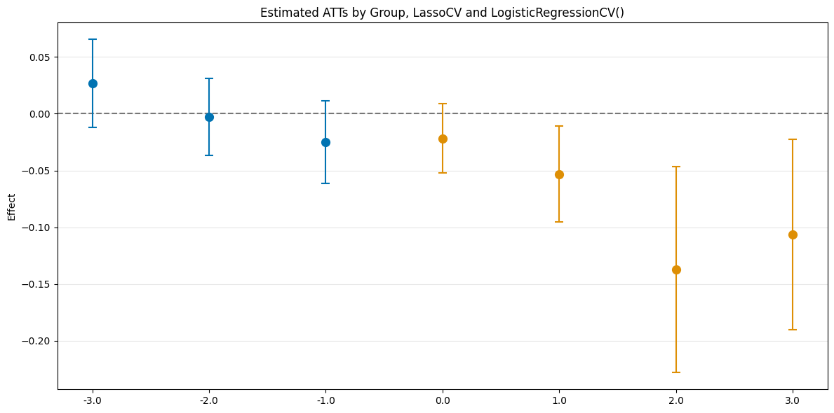
es_rf = dml_obj_lasso.aggregate("eventstudy")
es_rf.aggregated_frameworks.bootstrap()
es_rf.plot_effects(title="Estimated ATTs by Group, LassoCV and LogisticRegressionCV()")
[14]:
(<Figure size 1200x600 with 1 Axes>,
 <Axes: title={'center': 'Estimated ATTs by Group, LassoCV and LogisticRegressionCV()'}, ylabel='Effect'>)