Note
-
Download Jupyter notebook:
https://docs.doubleml.org/stable/examples/py_double_ml_cate.ipynb.
Python: Conditional Average Treatment Effects (CATEs) for IRM models#
In this simple example, we illustrate how the DoubleML package can be used to estimate conditional average treatment effects with B-splines for one or two-dimensional effects in the DoubleMLIRM model.
[1]:
import numpy as np
import pandas as pd
import doubleml as dml
from doubleml.irm.datasets import make_heterogeneous_data
Data#
We define a data generating process to create synthetic data to compare the estimates to the true effect. The data generating process is based on the Monte Carlo simulation from Oprescu et al. (2019).
The documentation of the data generating process can be found here.
One-dimensional Example#
We start with an one-dimensional effect and create our training data. In this example the true effect depends only the first covariate \(X_0\) and takes the following form
The generated dictionary also contains a callable with key treatment_effect to calculate the true treatment effect for new observations.
[2]:
np.random.seed(42)
data_dict = make_heterogeneous_data(
n_obs=2000,
p=10,
support_size=5,
n_x=1,
binary_treatment=True,
)
treatment_effect = data_dict['treatment_effect']
data = data_dict['data']
print(data.head())
y d X_0 X_1 X_2 X_3 X_4 X_5 \
0 4.803300 1.0 0.259828 0.886086 0.895690 0.297287 0.229994 0.411304
1 5.655547 1.0 0.824350 0.396992 0.156317 0.737951 0.360475 0.671271
2 1.878402 0.0 0.988421 0.977280 0.793818 0.659423 0.577807 0.866102
3 6.941440 1.0 0.427486 0.330285 0.564232 0.850575 0.201528 0.934433
4 1.703049 1.0 0.016200 0.818380 0.040139 0.889913 0.991963 0.294067
X_6 X_7 X_8 X_9
0 0.240532 0.672384 0.826065 0.673092
1 0.270644 0.081230 0.992582 0.156202
2 0.289440 0.467681 0.619390 0.411190
3 0.689088 0.823273 0.556191 0.779517
4 0.210319 0.765363 0.253026 0.865562
First, define the DoubleMLData object.
[3]:
data_dml_base = dml.DoubleMLData(
data,
y_col='y',
d_cols='d'
)
Next, define the learners for the nuisance functions and fit the IRM Model. Remark that linear learners would usually be optimal due to the data generating process.
[4]:
# First stage estimation
from sklearn.ensemble import RandomForestClassifier, RandomForestRegressor
randomForest_reg = RandomForestRegressor(n_estimators=500)
randomForest_class = RandomForestClassifier(n_estimators=500)
np.random.seed(42)
dml_irm = dml.DoubleMLIRM(data_dml_base,
ml_g=randomForest_reg,
ml_m=randomForest_class,
trimming_threshold=0.05,
n_folds=5)
print("Training IRM Model")
dml_irm.fit()
print(dml_irm.summary)
Training IRM Model
/tmp/ipykernel_46911/149446427.py:8: DeprecationWarning: 'trimming_threshold' is deprecated and will be removed in a future version. Use 'ps_processor_config' with 'clipping_threshold' instead.
dml_irm = dml.DoubleMLIRM(data_dml_base,
coef std err t P>|t| 2.5 % 97.5 %
d 4.475551 0.040813 109.658769 0.0 4.395558 4.555544
To estimate the CATE, we rely on the best-linear-predictor of the linear score as in Semenova et al. (2021) To approximate the target function \(\theta_0(x)\) with a linear form, we have to define a data frame of basis functions. Here, we rely on patsy to construct a suitable basis of B-splines.
[5]:
import patsy
design_matrix = patsy.dmatrix("bs(x, df=5, degree=2)", {"x": data["X_0"]})
spline_basis = pd.DataFrame(design_matrix)
To estimate the parameters to calculate the CATE estimate call the cate() method and supply the dataframe of basis elements.
[6]:
cate = dml_irm.cate(spline_basis)
print(cate)
================== DoubleMLBLP Object ==================
------------------ Fit summary ------------------
coef std err t P>|t| [0.025 0.975]
0 0.690968 0.143593 4.812003 1.494253e-06 0.409532 0.972405
1 2.302552 0.248178 9.277808 1.730011e-20 1.816131 2.788972
2 4.904976 0.161305 30.408135 4.288105e-203 4.588824 5.221127
3 4.756337 0.194167 24.496074 1.626530e-132 4.375776 5.136898
4 3.747008 0.195816 19.135309 1.283168e-81 3.363215 4.130802
5 4.314309 0.200042 21.566964 3.670051e-103 3.922232 4.706385
To obtain the confidence intervals for the CATE, we have to call the confint() method and a supply a dataframe of basis elements. This could be the same basis as for fitting the CATE model or a new basis to e.g. evaluate the CATE model on a grid. Here, we will evaluate the CATE on a grid from 0.1 to 0.9 to plot the final results. Further, we construct uniform confidence intervals by setting the option joint and providing a number of bootstrap repetitions n_rep_boot.
[7]:
new_data = {"x": np.linspace(0.1, 0.9, 100)}
spline_grid = pd.DataFrame(patsy.build_design_matrices([design_matrix.design_info], new_data)[0])
df_cate = cate.confint(spline_grid, level=0.95, joint=True, n_rep_boot=2000)
print(df_cate)
2.5 % effect 97.5 %
0 2.069634 2.333000 2.596367
1 2.185035 2.452622 2.720208
2 2.297102 2.570278 2.843454
3 2.406565 2.685970 2.965376
4 2.514024 2.799698 3.085372
.. ... ... ...
95 4.418052 4.705170 4.992288
96 4.424682 4.705682 4.986683
97 4.434116 4.708532 4.982948
98 4.445816 4.713719 4.981622
99 4.459098 4.721243 4.983389
[100 rows x 3 columns]
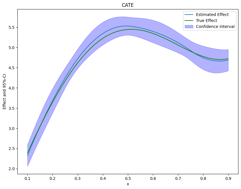
Finally, we can plot our results and compare them with the true effect.
[8]:
from matplotlib import pyplot as plt
plt.rcParams['figure.figsize'] = 10., 7.5
df_cate['x'] = new_data['x']
df_cate['true_effect'] = treatment_effect(new_data["x"].reshape(-1, 1))
fig, ax = plt.subplots()
ax.plot(df_cate['x'],df_cate['effect'], label='Estimated Effect')
ax.plot(df_cate['x'],df_cate['true_effect'], color="green", label='True Effect')
ax.fill_between(df_cate['x'], df_cate['2.5 %'], df_cate['97.5 %'], color='b', alpha=.3, label='Confidence Interval')
plt.legend()
plt.title('CATE')
plt.xlabel('x')
_ = plt.ylabel('Effect and 95%-CI')
If the effect is not one-dimensional, the estimate still corresponds to the projection of the true effect on the basis functions.
Two-Dimensional Example#
It is also possible to estimate multi-dimensional conditional effects. We will use a similar data generating process but now the effect depends on the first two covariates \(X_0\) and \(X_1\) and takes the following form
With the argument n_x=2 we can specify set the effect to be two-dimensional.
[9]:
np.random.seed(42)
data_dict = make_heterogeneous_data(
n_obs=5000,
p=10,
support_size=5,
n_x=2,
binary_treatment=True,
)
treatment_effect = data_dict['treatment_effect']
data = data_dict['data']
print(data.head())
y d X_0 X_1 X_2 X_3 X_4 X_5 \
0 1.286203 1.0 0.014080 0.006958 0.240127 0.100807 0.260211 0.177043
1 0.416899 1.0 0.152148 0.912230 0.892796 0.653901 0.672234 0.005339
2 2.087634 1.0 0.344787 0.893649 0.291517 0.562712 0.099731 0.921956
3 7.508433 1.0 0.619351 0.232134 0.000943 0.757151 0.985207 0.809913
4 0.567695 0.0 0.477130 0.447624 0.775191 0.526769 0.316717 0.258158
X_6 X_7 X_8 X_9
0 0.028520 0.909304 0.008223 0.736082
1 0.984872 0.877833 0.895106 0.659245
2 0.140770 0.224897 0.558134 0.764093
3 0.460207 0.903767 0.409848 0.524934
4 0.037747 0.583195 0.229961 0.148134
As univariate example estimate the IRM Model.
[10]:
data_dml_base = dml.DoubleMLData(
data,
y_col='y',
d_cols='d'
)
[11]:
# First stage estimation
from sklearn.ensemble import RandomForestClassifier, RandomForestRegressor
randomForest_reg = RandomForestRegressor(n_estimators=500)
randomForest_class = RandomForestClassifier(n_estimators=500)
np.random.seed(42)
dml_irm = dml.DoubleMLIRM(data_dml_base,
ml_g=randomForest_reg,
ml_m=randomForest_class,
trimming_threshold=0.05,
n_folds=5)
print("Training IRM Model")
dml_irm.fit()
print(dml_irm.summary)
Training IRM Model
/tmp/ipykernel_46911/149446427.py:8: DeprecationWarning: 'trimming_threshold' is deprecated and will be removed in a future version. Use 'ps_processor_config' with 'clipping_threshold' instead.
dml_irm = dml.DoubleMLIRM(data_dml_base,
coef std err t P>|t| 2.5 % 97.5 %
d 4.546967 0.038847 117.0473 0.0 4.470828 4.623107
As above, we will rely on the patsy package to construct the basis elements. In the two-dimensional case, we will construct a tensor product of B-splines (for more information see here).
[12]:
design_matrix = patsy.dmatrix("te(bs(x_0, df=7, degree=3), bs(x_1, df=7, degree=3))", {"x_0": data["X_0"], "x_1": data["X_1"]})
spline_basis = pd.DataFrame(design_matrix)
cate = dml_irm.cate(spline_basis)
print(cate)
================== DoubleMLBLP Object ==================
------------------ Fit summary ------------------
coef std err t P>|t| [0.025 0.975]
0 2.805714 0.142132 19.740200 9.739125e-87 2.527141 3.084288
1 -1.114258 0.830850 -1.341106 1.798862e-01 -2.742695 0.514179
2 0.460385 0.786429 0.585412 5.582705e-01 -1.080987 2.001758
3 2.311594 0.725142 3.187782 1.433684e-03 0.890342 3.732845
4 0.574050 0.739182 0.776601 4.373941e-01 -0.874721 2.022820
5 -3.333882 1.004192 -3.319965 9.002873e-04 -5.302062 -1.365702
6 -4.991824 1.104475 -4.519637 6.194588e-06 -7.156554 -2.827093
7 -6.405892 0.948828 -6.751372 1.464537e-11 -8.265562 -4.546223
8 -2.643988 0.809392 -3.266633 1.088346e-03 -4.230368 -1.057608
9 3.752522 0.855242 4.387673 1.145699e-05 2.076279 5.428766
10 -0.017605 0.725992 -0.024250 9.806532e-01 -1.440524 1.405313
11 1.577634 0.797410 1.978446 4.787838e-02 0.014738 3.140530
12 -1.072153 1.093173 -0.980771 3.267055e-01 -3.214732 1.070427
13 -2.296523 1.193581 -1.924061 5.434698e-02 -4.635900 0.042854
14 -2.606727 0.939390 -2.774915 5.521608e-03 -4.447897 -0.765557
15 0.240194 0.732307 0.327997 7.429141e-01 -1.195101 1.675489
16 1.088019 0.730823 1.488759 1.365509e-01 -0.344368 2.520406
17 3.741043 0.648094 5.772373 7.816296e-09 2.470801 5.011285
18 1.384717 0.676714 2.046238 4.073293e-02 0.058383 2.711051
19 -1.509005 0.912837 -1.653094 9.831167e-02 -3.298132 0.280122
20 -2.310097 1.013848 -2.278543 2.269425e-02 -4.297204 -0.322991
21 -2.805789 0.753136 -3.725477 1.949459e-04 -4.281908 -1.329671
22 1.945058 0.723958 2.686698 7.216215e-03 0.526125 3.363990
23 2.187732 0.754503 2.899568 3.736770e-03 0.708934 3.666530
24 4.375151 0.672266 6.508068 7.612328e-11 3.057535 5.692768
25 2.136010 0.649335 3.289536 1.003528e-03 0.863337 3.408682
26 1.709593 0.904900 1.889261 5.885686e-02 -0.063979 3.483165
27 -1.238287 0.981703 -1.261366 2.071771e-01 -3.162389 0.685816
28 -1.373783 0.848734 -1.618625 1.055280e-01 -3.037271 0.289706
29 4.063098 0.953706 4.260328 2.041275e-05 2.193870 5.932327
30 4.062774 0.886300 4.583969 4.562317e-06 2.325657 5.799890
31 6.077543 0.810564 7.497915 6.484111e-14 4.488866 7.666220
32 3.838322 0.778305 4.931646 8.153971e-07 2.312873 5.363771
33 2.586423 1.059936 2.440170 1.468035e-02 0.508988 4.663859
34 -1.845525 1.301629 -1.417859 1.562320e-01 -4.396671 0.705620
35 -0.431605 1.107809 -0.389603 6.968305e-01 -2.602870 1.739660
36 7.036381 1.008941 6.974023 3.080041e-12 5.058892 9.013870
37 5.191501 0.990838 5.239503 1.610093e-07 3.249494 7.133509
38 7.149681 0.831479 8.598753 8.058676e-18 5.520012 8.779349
39 6.735426 0.918044 7.336716 2.188986e-13 4.936094 8.534759
40 2.378471 1.181350 2.013350 4.407786e-02 0.063067 4.693874
41 4.441528 1.295590 3.428191 6.076187e-04 1.902219 6.980838
42 1.732983 1.094883 1.582803 1.134664e-01 -0.412947 3.878914
43 10.068340 1.002225 10.045991 9.568143e-24 8.104016 12.032664
44 3.734332 1.100664 3.392801 6.918199e-04 1.577071 5.891593
45 9.197356 0.697591 13.184449 1.078384e-39 7.830102 10.564610
46 5.366912 0.695860 7.712631 1.232497e-14 4.003051 6.730773
47 5.929031 0.816417 7.262261 3.806736e-13 4.328884 7.529178
48 1.296171 0.988081 1.311807 1.895853e-01 -0.640432 3.232774
49 1.238416 0.897115 1.380442 1.674507e-01 -0.519898 2.996729
Finally, we create a new grid to evaluate and plot the effects.
[13]:
grid_size = 100
x_0 = np.linspace(0.1, 0.9, grid_size)
x_1 = np.linspace(0.1, 0.9, grid_size)
x_0, x_1 = np.meshgrid(x_0, x_1)
new_data = {"x_0": x_0.ravel(), "x_1": x_1.ravel()}
[14]:
spline_grid = pd.DataFrame(patsy.build_design_matrices([design_matrix.design_info], new_data)[0])
df_cate = cate.confint(spline_grid, joint=True, n_rep_boot=2000)
print(df_cate)
2.5 % effect 97.5 %
0 1.671382 2.379892 3.088401
1 1.681261 2.367225 3.053188
2 1.698302 2.357450 3.016598
3 1.720409 2.350491 2.980574
4 1.745353 2.346274 2.947194
... ... ... ...
9995 3.715596 4.506833 5.298069
9996 3.830967 4.661521 5.492075
9997 3.938460 4.811763 5.685066
9998 4.041091 4.955689 5.870288
9999 4.141484 5.091432 6.041381
[10000 rows x 3 columns]
[15]:
import plotly.graph_objects as go
grid_array = np.array(list(zip(x_0.ravel(), x_1.ravel())))
true_effect = treatment_effect(grid_array).reshape(x_0.shape)
effect = np.asarray(df_cate['effect']).reshape(x_0.shape)
lower_bound = np.asarray(df_cate['2.5 %']).reshape(x_0.shape)
upper_bound = np.asarray(df_cate['97.5 %']).reshape(x_0.shape)
fig = go.Figure(data=[
go.Surface(x=x_0,
y=x_1,
z=true_effect),
go.Surface(x=x_0,
y=x_1,
z=upper_bound, showscale=False, opacity=0.4,colorscale='purp'),
go.Surface(x=x_0,
y=x_1,
z=lower_bound, showscale=False, opacity=0.4,colorscale='purp'),
])
fig.update_traces(contours_z=dict(show=True, usecolormap=True,
highlightcolor="limegreen", project_z=True))
fig.update_layout(scene = dict(
xaxis_title='X_0',
yaxis_title='X_1',
zaxis_title='Effect'),
width=700,
margin=dict(r=20, b=10, l=10, t=10))
fig.show()