Note
-
Download Jupyter notebook:
https://docs.doubleml.org/stable/examples/py_double_ml_cate_plr.ipynb.
Python: Conditional Average Treatment Effects (CATEs) for PLR models#
In this simple example, we illustrate how the DoubleML package can be used to estimate conditional average treatment effects with B-splines for one or two-dimensional effects in the DoubleMLPLR model.
[1]:
import numpy as np
import pandas as pd
import doubleml as dml
from doubleml.irm.datasets import make_heterogeneous_data
Data#
We define a data generating process to create synthetic data to compare the estimates to the true effect. The data generating process is based on the Monte Carlo simulation from Oprescu et al. (2019).
The documentation of the data generating process can be found here.
One-dimensional Example#
We start with an one-dimensional effect and create our training data. In this example the true effect depends only the first covariate \(X_0\) and takes the following form
The generated dictionary also contains a callable with key treatment_effect to calculate the true treatment effect for new observations.
[2]:
np.random.seed(42)
data_dict = make_heterogeneous_data(
n_obs=2000,
p=10,
support_size=5,
n_x=1,
)
treatment_effect = data_dict['treatment_effect']
data = data_dict['data']
print(data.head())
y d X_0 X_1 X_2 X_3 X_4 \
0 1.564451 0.241064 0.259828 0.886086 0.895690 0.297287 0.229994
1 1.114570 0.040912 0.824350 0.396992 0.156317 0.737951 0.360475
2 8.901013 1.392623 0.988421 0.977280 0.793818 0.659423 0.577807
3 -1.315155 -0.551317 0.427486 0.330285 0.564232 0.850575 0.201528
4 1.314625 0.683487 0.016200 0.818380 0.040139 0.889913 0.991963
X_5 X_6 X_7 X_8 X_9
0 0.411304 0.240532 0.672384 0.826065 0.673092
1 0.671271 0.270644 0.081230 0.992582 0.156202
2 0.866102 0.289440 0.467681 0.619390 0.411190
3 0.934433 0.689088 0.823273 0.556191 0.779517
4 0.294067 0.210319 0.765363 0.253026 0.865562
First, define the DoubleMLData object.
[3]:
data_dml_base = dml.DoubleMLData(
data,
y_col='y',
d_cols='d'
)
Next, define the learners for the nuisance functions and fit the PLR Model. Remark that linear learners would usually be optimal due to the data generating process.
[4]:
# First stage estimation
from sklearn.ensemble import RandomForestClassifier, RandomForestRegressor
ml_l = RandomForestRegressor(n_estimators=500)
ml_m = RandomForestRegressor(n_estimators=500)
np.random.seed(42)
dml_plr = dml.DoubleMLPLR(data_dml_base,
ml_l=ml_l,
ml_m=ml_m,
n_folds=5)
print("Training PLR Model")
dml_plr.fit()
print(dml_plr.summary)
Training PLR Model
coef std err t P>|t| 2.5 % 97.5 %
d 4.377572 0.043996 99.499416 0.0 4.291342 4.463803
To estimate the CATE, we rely on the best-linear-predictor of the linear score as in Semenova et al. (2021) To approximate the target function \(\theta_0(x)\) with a linear form, we have to define a data frame of basis functions. Here, we rely on patsy to construct a suitable basis of B-splines.
[5]:
import patsy
design_matrix = patsy.dmatrix("bs(x, df=5, degree=2)", {"x": data["X_0"]})
spline_basis = pd.DataFrame(design_matrix)
To estimate the parameters to calculate the CATE estimate call the cate() method and supply the dataframe of basis elements.
[6]:
cate = dml_plr.cate(spline_basis)
print(cate)
================== DoubleMLBLP Object ==================
------------------ Fit summary ------------------
coef std err t P>|t| [0.025 0.975]
0 1.238718 0.141069 8.780943 1.621097e-18 0.962228 1.515208
1 1.582290 0.237164 6.671717 2.528272e-11 1.117457 2.047123
2 4.179204 0.156209 26.753880 1.112867e-157 3.873039 4.485368
3 4.040067 0.180296 22.408000 3.288788e-111 3.686694 4.393441
4 3.275454 0.179810 18.216224 3.837366e-74 2.923033 3.627874
5 3.795008 0.182354 20.811255 3.422646e-96 3.437601 4.152414
To obtain the confidence intervals for the CATE, we have to call the confint() method and a supply a dataframe of basis elements. This could be the same basis as for fitting the CATE model or a new basis to e.g. evaluate the CATE model on a grid. Here, we will evaluate the CATE on a grid from 0.1 to 0.9 to plot the final results. Further, we construct uniform confidence intervals by setting the option joint and providing a number of bootstrap repetitions n_rep_boot.
[7]:
new_data = {"x": np.linspace(0.1, 0.9, 100)}
spline_grid = pd.DataFrame(patsy.build_design_matrices([design_matrix.design_info], new_data)[0])
df_cate = cate.confint(spline_grid, level=0.95, joint=True, n_rep_boot=2000)
print(df_cate)
2.5 % effect 97.5 %
0 2.199213 2.428779 2.658345
1 2.289198 2.521357 2.753516
2 2.376681 2.613391 2.850101
3 2.462473 2.704881 2.947290
4 2.547257 2.795828 3.044399
.. ... ... ...
95 4.495028 4.735713 4.976398
96 4.503768 4.738936 4.974104
97 4.514957 4.744125 4.973293
98 4.528145 4.751281 4.974416
99 4.542754 4.760403 4.978052
[100 rows x 3 columns]
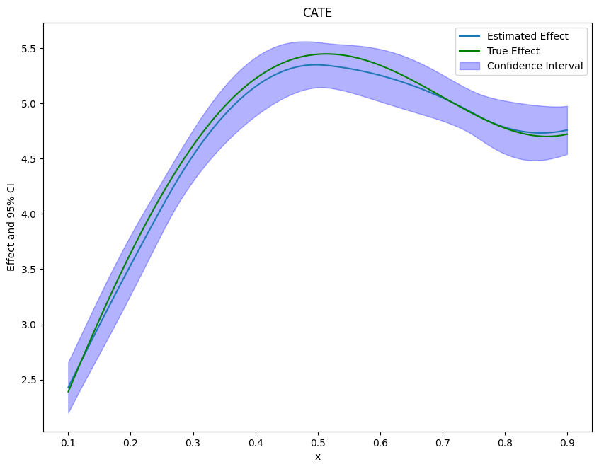
Finally, we can plot our results and compare them with the true effect.
[8]:
from matplotlib import pyplot as plt
plt.rcParams['figure.figsize'] = 10., 7.5
df_cate['x'] = new_data['x']
df_cate['true_effect'] = treatment_effect(new_data["x"].reshape(-1, 1))
fig, ax = plt.subplots()
ax.plot(df_cate['x'],df_cate['effect'], label='Estimated Effect')
ax.plot(df_cate['x'],df_cate['true_effect'], color="green", label='True Effect')
ax.fill_between(df_cate['x'], df_cate['2.5 %'], df_cate['97.5 %'], color='b', alpha=.3, label='Confidence Interval')
plt.legend()
plt.title('CATE')
plt.xlabel('x')
_ = plt.ylabel('Effect and 95%-CI')
If the effect is not one-dimensional, the estimate still corresponds to the projection of the true effect on the basis functions.
Two-Dimensional Example#
It is also possible to estimate multi-dimensional conditional effects. We will use a similar data generating process but now the effect depends on the first two covariates \(X_0\) and \(X_1\) and takes the following form
With the argument n_x=2 we can specify set the effect to be two-dimensional.
[9]:
np.random.seed(42)
data_dict = make_heterogeneous_data(
n_obs=5000,
p=10,
support_size=5,
n_x=2,
)
treatment_effect = data_dict['treatment_effect']
data = data_dict['data']
print(data.head())
y d X_0 X_1 X_2 X_3 X_4 \
0 -0.359307 -0.479722 0.014080 0.006958 0.240127 0.100807 0.260211
1 0.578557 -0.587135 0.152148 0.912230 0.892796 0.653901 0.672234
2 1.479882 0.172083 0.344787 0.893649 0.291517 0.562712 0.099731
3 4.468072 0.480579 0.619351 0.232134 0.000943 0.757151 0.985207
4 5.949866 0.974213 0.477130 0.447624 0.775191 0.526769 0.316717
X_5 X_6 X_7 X_8 X_9
0 0.177043 0.028520 0.909304 0.008223 0.736082
1 0.005339 0.984872 0.877833 0.895106 0.659245
2 0.921956 0.140770 0.224897 0.558134 0.764093
3 0.809913 0.460207 0.903767 0.409848 0.524934
4 0.258158 0.037747 0.583195 0.229961 0.148134
As univariate example estimate the PLR Model.
[10]:
data_dml_base = dml.DoubleMLData(
data,
y_col='y',
d_cols='d'
)
[11]:
# First stage estimation
from sklearn.ensemble import RandomForestClassifier, RandomForestRegressor
ml_l = RandomForestRegressor(n_estimators=500)
ml_m = RandomForestRegressor(n_estimators=500)
np.random.seed(42)
dml_plr = dml.DoubleMLPLR(data_dml_base,
ml_l=ml_l,
ml_m=ml_m,
n_folds=5)
print("Training PLR Model")
dml_plr.fit()
print(dml_plr.summary)
Training PLR Model
coef std err t P>|t| 2.5 % 97.5 %
d 4.470023 0.049729 89.886764 0.0 4.372555 4.567491
As above, we will rely on the patsy package to construct the basis elements. In the two-dimensional case, we will construct a tensor product of B-splines (for more information see here).
[12]:
design_matrix = patsy.dmatrix("te(bs(x_0, df=7, degree=3), bs(x_1, df=7, degree=3))", {"x_0": data["X_0"], "x_1": data["X_1"]})
spline_basis = pd.DataFrame(design_matrix)
cate = dml_plr.cate(spline_basis)
print(cate)
================== DoubleMLBLP Object ==================
------------------ Fit summary ------------------
coef std err t P>|t| [0.025 0.975]
0 2.784910 0.171860 16.204495 4.687227e-59 2.448070 3.121750
1 -3.322764 0.856037 -3.881567 1.037855e-04 -5.000565 -1.644963
2 3.063641 0.739261 4.144195 3.410095e-05 1.614716 4.512566
3 1.738422 0.719831 2.415040 1.573349e-02 0.327578 3.149265
4 2.013976 0.675528 2.981339 2.869912e-03 0.689967 3.337986
5 -3.883224 0.866142 -4.483357 7.347770e-06 -5.580831 -2.185617
6 -5.450097 0.933603 -5.837699 5.292652e-09 -7.279926 -3.620267
7 -7.349461 0.934122 -7.867775 3.610053e-15 -9.180307 -5.518616
8 -0.631113 0.797984 -0.790885 4.290112e-01 -2.195132 0.932906
9 -0.211682 0.825749 -0.256352 7.976791e-01 -1.830120 1.406756
10 1.903879 0.732162 2.600354 9.312769e-03 0.468869 3.338890
11 0.571040 0.705981 0.808860 4.185956e-01 -0.812658 1.954738
12 -0.870943 0.888348 -0.980407 3.268850e-01 -2.612073 0.870187
13 -1.232277 0.977113 -1.261140 2.072583e-01 -3.147383 0.682830
14 -2.158076 0.759373 -2.841920 4.484272e-03 -3.646419 -0.669733
15 0.084714 0.768874 0.110179 9.122671e-01 -1.422251 1.591679
16 2.891757 0.706173 4.094968 4.222264e-05 1.507683 4.275831
17 1.896333 0.639585 2.964940 3.027419e-03 0.642768 3.149897
18 2.686684 0.616346 4.359050 1.306282e-05 1.478668 3.894701
19 -1.997038 0.747977 -2.669919 7.586962e-03 -3.463046 -0.531030
20 -1.962022 0.758852 -2.585513 9.723414e-03 -3.449345 -0.474699
21 -4.130609 0.631179 -6.544276 5.978438e-11 -5.367697 -2.893521
22 0.159592 0.788896 0.202298 8.396835e-01 -1.386616 1.705801
23 4.431747 0.767486 5.774365 7.724375e-09 2.927501 5.935993
24 2.308837 0.714261 3.232485 1.227184e-03 0.908912 3.708762
25 3.344463 0.683785 4.891102 1.002728e-06 2.004269 4.684657
26 0.030817 0.810833 0.038006 9.696826e-01 -1.558387 1.620021
27 -1.188545 0.887270 -1.339553 1.803908e-01 -2.927563 0.550472
28 -1.133676 0.916355 -1.237158 2.160285e-01 -2.929699 0.662347
29 5.561652 1.259230 4.416709 1.002149e-05 3.093607 8.029696
30 1.409551 1.078382 1.307098 1.911794e-01 -0.704039 3.523140
31 7.400297 0.959441 7.713137 1.227621e-14 5.519828 9.280766
32 2.915502 0.911818 3.197462 1.386428e-03 1.128372 4.702632
33 2.222430 1.087826 2.043002 4.105227e-02 0.090331 4.354529
34 0.207242 1.155995 0.179276 8.577210e-01 -2.058467 2.472952
35 1.047390 1.062293 0.985971 3.241474e-01 -1.034666 3.129446
36 6.559844 1.290507 5.083153 3.712209e-07 4.030497 9.089191
37 5.129085 1.224822 4.187617 2.818990e-05 2.728478 7.529692
38 7.066039 0.962041 7.344845 2.059976e-13 5.180474 8.951604
39 5.936238 1.178273 5.038085 4.702119e-07 3.626866 8.245610
40 4.313796 1.355564 3.182288 1.461162e-03 1.656939 6.970652
41 1.631762 1.329967 1.226919 2.198529e-01 -0.974925 4.238449
42 -0.758754 1.390495 -0.545672 5.852916e-01 -3.484074 1.966566
43 8.390312 1.384755 6.059058 1.369212e-09 5.676242 11.104383
44 7.240053 1.560250 4.640314 3.478794e-06 4.182018 10.298088
45 8.034609 0.912801 8.802149 1.342214e-18 6.245552 9.823666
46 7.023728 1.135398 6.186136 6.165670e-10 4.798388 9.249067
47 4.663357 1.331161 3.503226 4.596588e-04 2.054330 7.272384
48 2.479527 0.934634 2.652940 7.979409e-03 0.647679 4.311375
49 3.650893 0.538227 6.783183 1.175564e-11 2.595987 4.705798
Finally, we create a new grid to evaluate and plot the effects.
[13]:
grid_size = 100
x_0 = np.linspace(0.1, 0.9, grid_size)
x_1 = np.linspace(0.1, 0.9, grid_size)
x_0, x_1 = np.meshgrid(x_0, x_1)
new_data = {"x_0": x_0.ravel(), "x_1": x_1.ravel()}
[14]:
spline_grid = pd.DataFrame(patsy.build_design_matrices([design_matrix.design_info], new_data)[0])
df_cate = cate.confint(spline_grid, joint=True, n_rep_boot=2000)
print(df_cate)
2.5 % effect 97.5 %
0 1.333947 2.035579 2.737210
1 1.349867 2.035735 2.721604
2 1.376972 2.042517 2.708062
3 1.412919 2.055410 2.697900
4 1.455262 2.073900 2.692538
... ... ... ...
9995 3.544680 4.252849 4.961018
9996 3.583140 4.333973 5.084807
9997 3.620135 4.417619 5.215103
9998 3.660360 4.504076 5.347793
9999 3.708154 4.593637 5.479119
[10000 rows x 3 columns]
[15]:
import plotly.graph_objects as go
grid_array = np.array(list(zip(x_0.ravel(), x_1.ravel())))
true_effect = treatment_effect(grid_array).reshape(x_0.shape)
effect = np.asarray(df_cate['effect']).reshape(x_0.shape)
lower_bound = np.asarray(df_cate['2.5 %']).reshape(x_0.shape)
upper_bound = np.asarray(df_cate['97.5 %']).reshape(x_0.shape)
fig = go.Figure(data=[
go.Surface(x=x_0,
y=x_1,
z=true_effect),
go.Surface(x=x_0,
y=x_1,
z=upper_bound, showscale=False, opacity=0.4,colorscale='purp'),
go.Surface(x=x_0,
y=x_1,
z=lower_bound, showscale=False, opacity=0.4,colorscale='purp'),
])
fig.update_traces(contours_z=dict(show=True, usecolormap=True,
highlightcolor="limegreen", project_z=True))
fig.update_layout(scene = dict(
xaxis_title='X_0',
yaxis_title='X_1',
zaxis_title='Effect'),
width=700,
margin=dict(r=20, b=10, l=10, t=10))
fig.show()