Note

Download Jupyter notebook: https://docs.doubleml.org/stable/examples/R_double_ml_pension.ipynb.

R: Impact of 401(k) on Financial Wealth

In this real-data example, we illustrate how the DoubleML package can be used to estimate the effect of 401(k) eligibility and participation on accumulated assets. The 401(k) data set has been analyzed in several studies, among others Chernozhukov et al. (2018).

401(k) plans are pension accounts sponsored by employers. The key problem in determining the effect of participation in 401(k) plans on accumulated assets is saver heterogeneity coupled with the fact that the decision to enroll in a 401(k) is non-random. It is generally recognized that some people have a higher preference for saving than others. It also seems likely that those individuals with high unobserved preference for saving would be most likely to choose to participate in tax-advantaged retirement savings plans and would tend to have otherwise high amounts of accumulated assets. The presence of unobserved savings preferences with these properties then implies that conventional estimates that do not account for saver heterogeneity and endogeneity of participation will be biased upward, tending to overstate the savings effects of 401(k) participation.

One can argue that eligibility for enrolling in a 401(k) plan in this data can be taken as exogenous after conditioning on a few observables of which the most important for their argument is income. The basic idea is that, at least around the time 401(k)’s initially became available, people were unlikely to be basing their employment decisions on whether an employer offered a 401(k) but would instead focus on income and other aspects of the job.

Data

The preprocessed data can be fetched by calling fetch_401k(). The arguments polynomial_features and instrument can be used to replicate the models used in Chernozhukov et al. (2018). Note that an internet connection is required for loading the data. We start with a baseline specification of the regression model and reload the data later in case we want to use another specification.

# Load required packages for this tutorial
library(DoubleML)
library(mlr3)
library(mlr3learners)
library(data.table)
library(ggplot2)

# suppress messages during fitting
lgr::get_logger("mlr3")$set_threshold("warn")

# load data as a data.table
data = fetch_401k(return_type = "data.table", instrument = TRUE)
dim(data)
str(data)

Warning message:
"Paket 'mlr3' wurde unter R Version 4.2.3 erstellt"

1. 9915
2. 12

Classes 'data.table' and 'data.frame':  9915 obs. of  12 variables:
 $ net_tfa: num  0 1015 -2000 15000 0 ...
 $ age    : num  47 36 37 58 32 34 28 54 43 32 ...
 $ inc    : num  6765 28452 3300 52590 21804 ...
 $ educ   : num  8 16 12 16 11 16 12 11 14 18 ...
 $ fsize  : num  2 1 6 2 1 1 3 3 2 3 ...
 $ marr   : num  0 0 0 1 0 0 1 0 1 1 ...
 $ twoearn: num  0 0 0 1 0 0 1 0 1 0 ...
 $ db     : num  0 0 1 0 0 0 0 0 1 0 ...
 $ pira   : num  0 0 0 0 0 1 1 0 1 0 ...
 $ hown   : num  1 1 0 1 1 1 1 1 1 1 ...
 $ p401   : int  0 0 0 0 0 0 0 0 0 0 ...
 $ e401   : int  0 0 0 0 0 0 0 0 0 0 ...
 - attr(*, ".internal.selfref")=<externalptr>

See the “Details” section on the description of the data set, which can be accessed by typing help(fetch_401k).

The data consist of 9,915 observations at the household level drawn from the 1991 Survey of Income and Program Participation (SIPP). All the variables are referred to 1990. We use net financial assets (net_tfa) as the outcome variable, \(Y\), in our analysis. The net financial assets are computed as the sum of IRA balances, 401(k) balances, checking accounts, saving bonds, other interest-earning accounts, other interest-earning assets, stocks, and mutual funds less non mortgage debts.

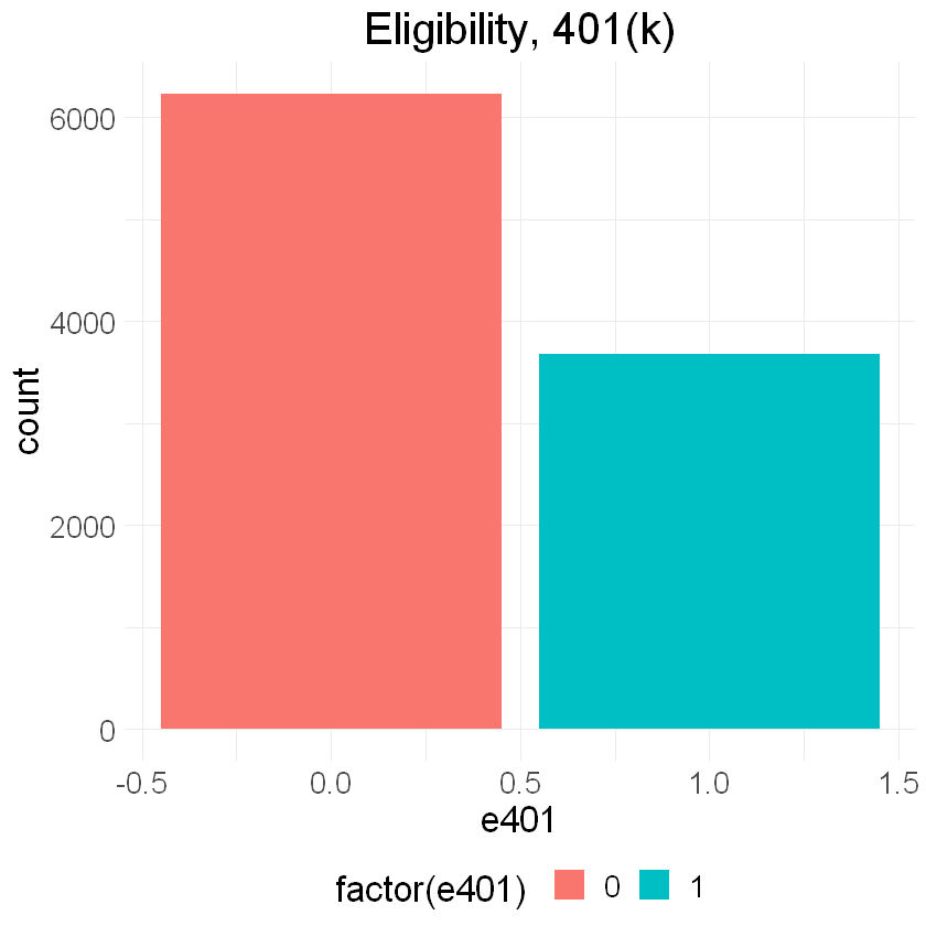
Among the \(9915\) individuals, \(3682\) are eligible to participate in the program. The variable e401 indicates eligibility and p401 indicates participation, respectively.

hist_e401 = ggplot(data, aes(x = e401, fill = factor(e401))) +
            geom_bar() + theme_minimal() +
            ggtitle("Eligibility, 401(k)") +
            theme(legend.position = "bottom", plot.title = element_text(hjust = 0.5),
                  text = element_text(size = 20))
hist_e401

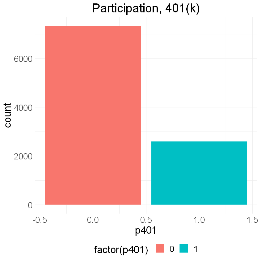
hist_p401 = ggplot(data, aes(x = p401, fill = factor(p401))) +
            geom_bar() + theme_minimal() +
            ggtitle("Participation, 401(k)") +
            theme(legend.position = "bottom", plot.title = element_text(hjust = 0.5),
                  text = element_text(size = 20))
hist_p401

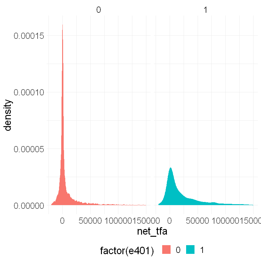
Eligibility is highly associated with financial wealth:

dens_net_tfa = ggplot(data, aes(x = net_tfa, color = factor(e401), fill = factor(e401)) ) +
                    geom_density() + xlim(c(-20000, 150000)) +
                    facet_wrap(.~e401)  + theme_minimal() +
                    theme(legend.position = "bottom", text = element_text(size = 20))

dens_net_tfa

Warning message:
"Removed 340 rows containing non-finite values (`stat_density()`)."

As a first estimate, we calculate the unconditional average predictive effect (APE) of 401(k) eligibility on accumulated assets. This effect corresponds to the average treatment effect if 401(k) eligibility would be assigned to individuals in an entirely randomized way. The unconditional APE of e401 is about \(19559\):

APE_e401_uncond = data[e401==1, mean(net_tfa)] - data[e401==0, mean(net_tfa)]
round(APE_e401_uncond, 2)

19559.34

Among the \(3682\) individuals that are eligible, \(2594\) decided to participate in the program. The unconditional APE of p401 is about \(27372\):

APE_p401_uncond = data[p401==1, mean(net_tfa)] - data[p401==0, mean(net_tfa)]
round(APE_p401_uncond, 2)

27371.58

As discussed, these estimates are biased since they do not account for saver heterogeneity and endogeneity of participation.

The DoubleML package

Let’s use the package DoubleML to estimate the average treatment effect of 401(k) eligibility, i.e. e401, and participation, i.e. p401, on net financial assets net_tfa.

Estimating the Average Treatment Effect of 401(k) Eligibility on Net Financial Assets

We first look at the treatment effect of e401 on net total financial assets. We give estimates of the ATE in the linear model

\begin{equation*} Y = D \alpha + f(X)'\beta+ \epsilon, \end{equation*} where \(f(X)\) is a dictonary applied to the raw regressors. \(X\) contains variables on marital status, two-earner status, defined benefit pension status, IRA participation, home ownership, family size, education, age, and income.

In the following, we will consider two different models,

• a basic model specification that includes the raw regressors, i.e., \(f(X) = X\), and

• a flexible model specification, where \(f(X)\) includes the raw regressors \(X\) and the orthogonal polynomials of degree 2 for the variables family size education, age, and income.

We will use the basic model specification whenever we use nonlinear methods, for example regression trees or random forests, and use the flexible model for linear methods such as the lasso. There are, of course, multiple ways how the model can be specified even more flexibly, for example including interactions of variable and higher order interaction. However, for the sake of simplicity we stick to the specification above. Users who are interested in varying the model can manipulate the model formula below (formula_flex), for example implementing the orignal specification in Chernozhukov et al. (2018).

In the first step, we report estimates of the average treatment effect (ATE) of 401(k) eligibility on net financial assets both in the partially linear regression (PLR) model and in the interactive regression model (IRM) allowing for heterogeneous treatment effects.

The Data Backend: DoubleMLData

To start our analysis, we initialize the data backend, i.e., a new instance of a DoubleMLData object. Here, we manually implement the regression model by using R’s formula interface. A shortcut would be to directly specify the options polynomial_features and instrument when calling fetch_401k().\(^{**}\)

To implement both models (basic and flexible), we generate two data backends: data_dml_base and data_dml_flex.

\(^{**}\) Note that the model specification using polynomial_features differs from the one used in our example.

# Set up basic model: Specify variables for data-backend
features_base = c("age", "inc", "educ", "fsize",
                  "marr", "twoearn", "db", "pira", "hown")

# Initialize DoubleMLData (data-backend of DoubleML)
data_dml_base = DoubleMLData$new(data,
                                 y_col = "net_tfa",
                                 d_cols = "e401",
                                 x_cols = features_base)
data_dml_base

================= DoubleMLData Object ==================


------------------ Data summary      ------------------
Outcome variable: net_tfa
Treatment variable(s): e401
Covariates: age, inc, educ, fsize, marr, twoearn, db, pira, hown
Instrument(s):
No. Observations: 9915

# Set up a model according to regression formula with polynomials
formula_flex = formula(" ~ -1 + poly(age, 2, raw=TRUE) +
                        poly(inc, 2, raw=TRUE) + poly(educ, 2, raw=TRUE) +
                        poly(fsize, 2, raw=TRUE) + marr + twoearn +
                        db + pira + hown")
features_flex = data.frame(model.matrix(formula_flex, data))

model_data = data.table("net_tfa" = data[, net_tfa],
                        "e401" = data[, e401],
                        features_flex)

# Initialize DoubleMLData (data-backend of DoubleML)
data_dml_flex = DoubleMLData$new(model_data,
                                 y_col = "net_tfa",
                                 d_cols = "e401")

data_dml_flex

================= DoubleMLData Object ==================


------------------ Data summary      ------------------
Outcome variable: net_tfa
Treatment variable(s): e401
Covariates: poly.age..2..raw...TRUE.1, poly.age..2..raw...TRUE.2, poly.inc..2..raw...TRUE.1, poly.inc..2..raw...TRUE.2, poly.educ..2..raw...TRUE.1, poly.educ..2..raw...TRUE.2, poly.fsize..2..raw...TRUE.1, poly.fsize..2..raw...TRUE.2, marr, twoearn, db, pira, hown
Instrument(s):
No. Observations: 9915

Partially Linear Regression Model (PLR)

We start using lasso to estimate the function \(g_0\) and \(m_0\) in the following PLR model:

\begin{eqnarray} & Y = D\theta_0 + g_0(X) + \zeta, &\quad E[\zeta \mid D,X]= 0,\\ & D = m_0(X) + V, &\quad E[V \mid X] = 0. \end{eqnarray}

To estimate the causal parameter \(\theta_0\) here, we use double machine learning with 3-fold cross-fitting.

Estimation of the nuisance components \(g_0\) and \(m_0\), is based on the lasso with cross-validated choice of the penalty term , \(\lambda\), as provided by the glmnet package. We load the learner by using the mlr3 function lrn(). Hyperparameters and options can be set during instantiation of the learner. Here we specify that the lasso should use that value of \(\lambda\) that minimizes the cross-validated mean squared error which is based on 5-fold cross validation.

In order to use a learner, the underlying R packages have to be installed. In this case, the package glmnet package needs to be installed. Moreover, installation of the package mlr3learners is required.

We start by estimation the ATE in the basic model and then repeat the estimation in the flexible model.

# Initialize learners
set.seed(123)
lasso = lrn("regr.cv_glmnet", nfolds = 5, s = "lambda.min")
lasso_class = lrn("classif.cv_glmnet", nfolds = 5, s = "lambda.min")

# Initialize DoubleMLPLR model
dml_plr_lasso = DoubleMLPLR$new(data_dml_base,
                                ml_l = lasso,
                                ml_m = lasso_class,
                                n_folds = 3)
dml_plr_lasso$fit()
dml_plr_lasso$summary()

Estimates and significance testing of the effect of target variables
     Estimate. Std. Error t value Pr(>|t|)
e401      6133       1465   4.185 2.85e-05 ***
---
Signif. codes:  0 '***' 0.001 '**' 0.01 '*' 0.05 '.' 0.1 ' ' 1

# Initialize learners
set.seed(123)
lasso = lrn("regr.cv_glmnet", nfolds = 5, s = "lambda.min")
lasso_class = lrn("classif.cv_glmnet", nfolds = 5, s = "lambda.min")

# Initialize DoubleMLPLR model
dml_plr_lasso = DoubleMLPLR$new(data_dml_flex,
                                ml_l = lasso,
                                ml_m = lasso_class,
                                n_folds = 3)
dml_plr_lasso$fit()
dml_plr_lasso$summary()

Estimates and significance testing of the effect of target variables
     Estimate. Std. Error t value Pr(>|t|)
e401      9580       1325   7.229 4.87e-13 ***
---
Signif. codes:  0 '***' 0.001 '**' 0.01 '*' 0.05 '.' 0.1 ' ' 1

Alternatively, we can repeat this procedure with other machine learning methods, for example a random forest learner as provided by the ranger package for R. The website of the mlr3extralearners package has a searchable list of all learners that are available in the mlr3verse.

# Random Forest
randomForest = lrn("regr.ranger", max.depth = 7,
                   mtry = 3, min.node.size = 3)
randomForest_class = lrn("classif.ranger", max.depth = 5,
                         mtry = 4, min.node.size = 7)

set.seed(123)
dml_plr_forest = DoubleMLPLR$new(data_dml_base,
                                 ml_l = randomForest,
                                 ml_m = randomForest_class,
                                 n_folds = 3)
dml_plr_forest$fit()
dml_plr_forest$summary()

Estimates and significance testing of the effect of target variables
     Estimate. Std. Error t value Pr(>|t|)
e401      9127       1313   6.952 3.61e-12 ***
---
Signif. codes:  0 '***' 0.001 '**' 0.01 '*' 0.05 '.' 0.1 ' ' 1

Now, let’s use a regression tree as provided by the R package rpart.

# Trees
trees = lrn("regr.rpart", cp = 0.0047, minsplit = 203)
trees_class = lrn("classif.rpart", cp = 0.0042, minsplit = 104)

set.seed(123)
dml_plr_tree = DoubleMLPLR$new(data_dml_base,
                               ml_l = trees,
                               ml_m = trees_class,
                               n_folds = 3)
dml_plr_tree$fit()
dml_plr_tree$summary()

Estimates and significance testing of the effect of target variables
     Estimate. Std. Error t value Pr(>|t|)
e401      8210       1324   6.203 5.55e-10 ***
---
Signif. codes:  0 '***' 0.001 '**' 0.01 '*' 0.05 '.' 0.1 ' ' 1

We can also experiment with extreme gradient boosting as provided by xgboost.

# Boosted trees
boost = lrn("regr.xgboost",
            objective = "reg:squarederror",
            eta = 0.1, nrounds = 35)
boost_class = lrn("classif.xgboost",
                  objective = "binary:logistic", eval_metric = "logloss",
                  eta = 0.1, nrounds = 34)

set.seed(123)
dml_plr_boost = DoubleMLPLR$new(data_dml_base,
                                ml_l = boost,
                                ml_m = boost_class,
                                n_folds = 3)
dml_plr_boost$fit()
dml_plr_boost$summary()

Estimates and significance testing of the effect of target variables
     Estimate. Std. Error t value Pr(>|t|)
e401      8700       1360   6.399 1.57e-10 ***
---
Signif. codes:  0 '***' 0.001 '**' 0.01 '*' 0.05 '.' 0.1 ' ' 1

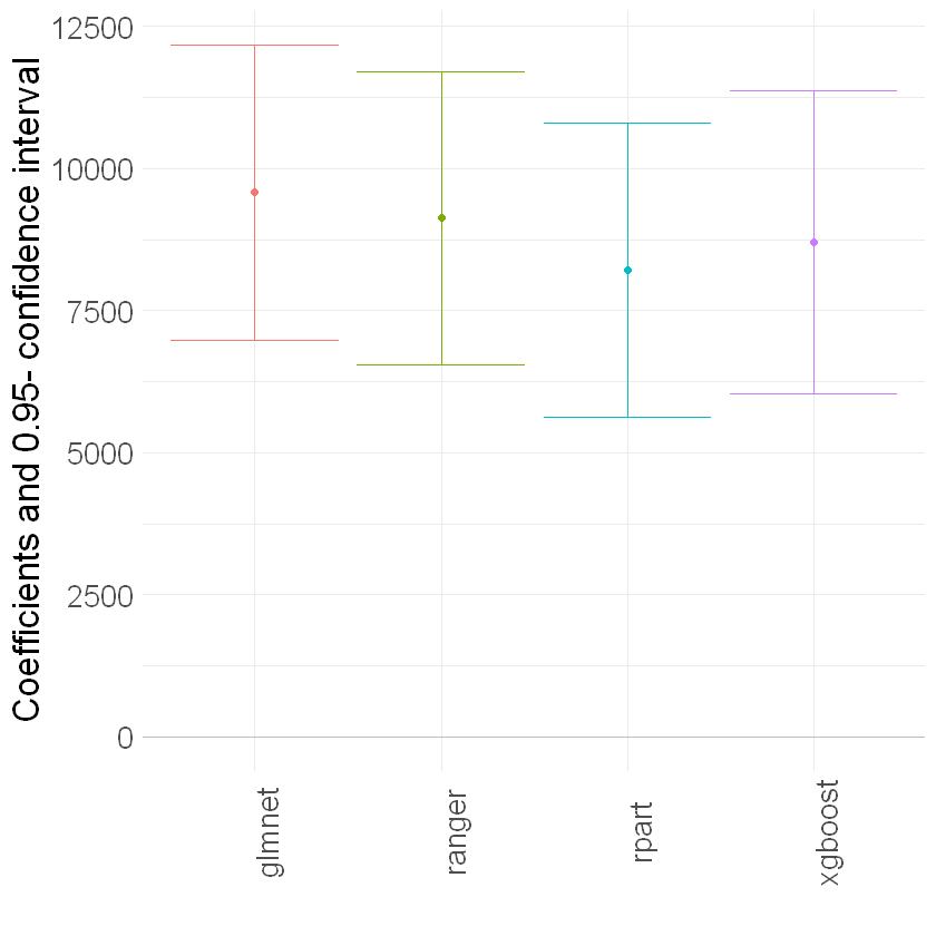
Let’s sum up the results:

confints = rbind(dml_plr_lasso$confint(), dml_plr_forest$confint(),
                 dml_plr_tree$confint(), dml_plr_boost$confint())
estimates = c(dml_plr_lasso$coef, dml_plr_forest$coef,
              dml_plr_tree$coef, dml_plr_boost$coef)
result_plr = data.table("model" = "PLR",
                        "ML" = c("glmnet", "ranger", "rpart", "xgboost"),
                        "Estimate" = estimates,
                        "lower" = confints[,1],
                        "upper" = confints[,2])
result_plr

A data.table: 4 × 5

model	ML	Estimate	lower	upper
<chr>	<chr>	<dbl>	<dbl>	<dbl>
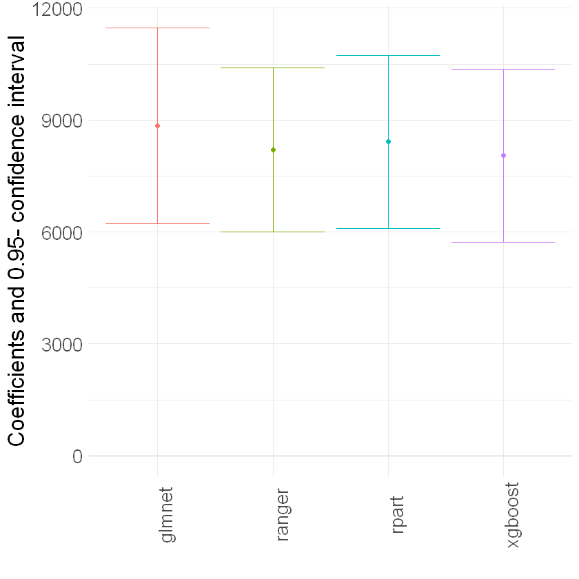
PLR	glmnet	9579.771	6982.443	12177.10
PLR	ranger	9126.999	6553.684	11700.31
PLR	rpart	8209.737	5615.525	10803.95
PLR	xgboost	8700.134	6035.281	11364.99

g_ci = ggplot(result_plr, aes(x = ML, y = Estimate, color = ML)) +
        geom_point() +
        geom_errorbar(aes(ymin = lower, ymax = upper, color = ML))  +
        geom_hline(yintercept = 0, color = "grey") +
        theme_minimal() + ylab("Coefficients and 0.95- confidence interval") +
        xlab("") +
        theme(axis.text.x = element_text(angle = 90), legend.position = "none",
              text = element_text(size = 20))

g_ci

Interactive Regression Model (IRM)

Next, we consider estimation of average treatment effects when treatment effects are fully heterogeneous:

\begin{eqnarray} & Y = g_0(D,X) + U, &\quad E[U\mid X,D] = 0,\\ & D = m_0(X) + V, &\quad E[V\mid X] = 0. \end{eqnarray}

To reduce the disproportionate impact of extreme propensity score weights in the interactive model we trim the propensity scores which are close to the bounds.

set.seed(123)
# Initialize DoubleMLIRM model
dml_irm_lasso = DoubleMLIRM$new(data_dml_flex,
                                ml_g = lasso,
                                ml_m = lasso_class,
                                trimming_threshold = 0.01,
                                n_folds = 3)
dml_irm_lasso$fit()
dml_irm_lasso$summary()

Estimates and significance testing of the effect of target variables
     Estimate. Std. Error t value Pr(>|t|)
e401      8850       1341   6.601 4.08e-11 ***
---
Signif. codes:  0 '***' 0.001 '**' 0.01 '*' 0.05 '.' 0.1 ' ' 1

# Initialize Learner
randomForest = lrn("regr.ranger")
randomForest_class = lrn("classif.ranger")

# Random Forest
set.seed(123)
dml_irm_forest = DoubleMLIRM$new(data_dml_base,
                                 ml_g = randomForest,
                                 ml_m = randomForest_class,
                                 trimming_threshold = 0.01,
                                 n_folds = 3)

# Set nuisance-part specific parameters
dml_irm_forest$set_ml_nuisance_params(
    "ml_g0", "e401", list(max.depth = 6, mtry = 4, min.node.size = 7))
dml_irm_forest$set_ml_nuisance_params(
    "ml_g1", "e401", list(max.depth = 6, mtry = 3, min.node.size = 5))
dml_irm_forest$set_ml_nuisance_params(
    "ml_m", "e401", list(max.depth = 6, mtry = 3, min.node.size = 6))

dml_irm_forest$fit()
dml_irm_forest$summary()

Estimates and significance testing of the effect of target variables
     Estimate. Std. Error t value Pr(>|t|)
e401      8202       1118   7.334 2.23e-13 ***
---
Signif. codes:  0 '***' 0.001 '**' 0.01 '*' 0.05 '.' 0.1 ' ' 1

# Initialize Learner
trees = lrn("regr.rpart")
trees_class = lrn("classif.rpart")

# Trees
set.seed(123)
dml_irm_tree = DoubleMLIRM$new(data_dml_base,
                          ml_g = trees,
                          ml_m = trees_class,
                          trimming_threshold = 0.01,
                          n_folds = 3)

# Set nuisance-part specific parameters
dml_irm_tree$set_ml_nuisance_params(
    "ml_g0", "e401", list(cp = 0.0016, minsplit = 74))
dml_irm_tree$set_ml_nuisance_params(
    "ml_g1", "e401", list(cp = 0.0018, minsplit = 70))
dml_irm_tree$set_ml_nuisance_params(
    "ml_m", "e401", list(cp = 0.0028, minsplit = 167))

dml_irm_tree$fit()
dml_irm_tree$summary()

Estimates and significance testing of the effect of target variables
     Estimate. Std. Error t value Pr(>|t|)
e401      8415       1186   7.098 1.26e-12 ***
---
Signif. codes:  0 '***' 0.001 '**' 0.01 '*' 0.05 '.' 0.1 ' ' 1

# Initialize Learners
boost = lrn("regr.xgboost", objective = "reg:squarederror")
boost_class = lrn("classif.xgboost", objective = "binary:logistic", eval_metric = "logloss")

# Boosted Trees
set.seed(123)
dml_irm_boost = DoubleMLIRM$new(data_dml_base,
                                ml_g = boost,
                                ml_m = boost_class,
                                trimming_threshold = 0.01,
                                n_folds = 3)

# Set nuisance-part specific parameters
if (compareVersion(as.character(packageVersion("DoubleML")), "0.2.1") > 0) {
    dml_irm_boost$set_ml_nuisance_params(
        "ml_g0", "e401", list(nrounds = 8, eta = 0.1))
    dml_irm_boost$set_ml_nuisance_params(
        "ml_g1", "e401", list(nrounds = 29, eta = 0.1))
    dml_irm_boost$set_ml_nuisance_params(
        "ml_m", "e401", list(nrounds = 23, eta = 0.1))
} else {
    # behavior of set_ml_nuisance_params() changed in https://github.com/DoubleML/doubleml-for-r/pull/89
    dml_irm_boost$set_ml_nuisance_params(
        "ml_g0", "e401", list(nrounds = 8, eta = 0.1, objective = "reg:squarederror", verbose=0))
    dml_irm_boost$set_ml_nuisance_params(
        "ml_g1", "e401", list(nrounds = 29, eta = 0.1, objective = "reg:squarederror", verbose=0))
    dml_irm_boost$set_ml_nuisance_params(
        "ml_m", "e401", list(nrounds = 23, eta = 0.1, objective = "binary:logistic", eval_metric = "logloss", verbose=0))
}

dml_irm_boost$fit()
dml_irm_boost$summary()

Estimates and significance testing of the effect of target variables
     Estimate. Std. Error t value Pr(>|t|)
e401      8048       1182   6.808 9.91e-12 ***
---
Signif. codes:  0 '***' 0.001 '**' 0.01 '*' 0.05 '.' 0.1 ' ' 1

confints = rbind(dml_irm_lasso$confint(), dml_irm_forest$confint(),
                 dml_irm_tree$confint(), dml_irm_boost$confint())
estimates = c(dml_irm_lasso$coef, dml_irm_forest$coef,
              dml_irm_tree$coef, dml_irm_boost$coef)
result_irm = data.table("model" = "IRM",
                        "ML" = c("glmnet", "ranger", "rpart", "xgboost"),
                        "Estimate" = estimates,
                        "lower" = confints[,1],
                        "upper" = confints[,2])
result_irm

g_ci = ggplot(result_irm, aes(x = ML, y = Estimate, color = ML)) +
        geom_point() +
        geom_errorbar(aes(ymin = lower, ymax = upper, color = ML))  +
        geom_hline(yintercept = 0, color = "grey") +
        theme_minimal() + ylab("Coefficients and 0.95- confidence interval") +
        xlab("") +
        theme(axis.text.x = element_text(angle = 90), legend.position = "none",
              text = element_text(size = 20))

g_ci

A data.table: 4 × 5

model	ML	Estimate	lower	upper
<chr>	<chr>	<dbl>	<dbl>	<dbl>
IRM	glmnet	8850.064	6222.396	11477.73
IRM	ranger	8202.101	6010.245	10393.96
IRM	rpart	8415.276	6091.618	10738.93
IRM	xgboost	8047.598	5730.684	10364.51

These estimates that flexibly account for confounding are substantially attenuated relative to the baseline estimate (19559) that does not account for confounding. They suggest much smaller causal effects of 401(k) eligiblity on financial asset holdings.

Local Average Treatment Effects of 401(k) Participation on Net Financial Assets

Interactive IV Model (IIVM)

In the examples above, we estimated the average treatment effect of eligibility on financial asset holdings. Now, we consider estimation of local average treatment effects (LATE) of participation using eligibility as an instrument for the participation decision. Under appropriate assumptions, the LATE identifies the treatment effect for so-called compliers, i.e., individuals who would only participate if eligible and otherwise not participate in the program.

As before, \(Y\) denotes the outcome net_tfa, and \(X\) is the vector of covariates. We use e401 as a binary instrument for the treatment variable p401. Here the structural equation model is:

\begin{eqnarray} & Y = g_0(Z,X) + U, &\quad E[U\mid Z,X] = 0,\\ & D = r_0(Z,X) + V, &\quad E[V\mid Z, X] = 0,\\ & Z = m_0(X) + \zeta, &\quad E[\zeta \mid X] = 0. \end{eqnarray}

# Initialize DoubleMLData with an instrument

# Basic model
data_dml_base_iv = DoubleMLData$new(data,
                                    y_col = "net_tfa",
                                    d_cols = "p401",
                                    x_cols = features_base,
                                    z_cols = "e401")
data_dml_base_iv

================= DoubleMLData Object ==================


------------------ Data summary      ------------------
Outcome variable: net_tfa
Treatment variable(s): p401
Covariates: age, inc, educ, fsize, marr, twoearn, db, pira, hown
Instrument(s): e401
No. Observations: 9915

# Flexible model
model_data = data.table("net_tfa" = data[, net_tfa],
                        "e401" = data[, e401],
                        "p401" = data[, p401],
                        features_flex)
data_dml_flex_iv = DoubleMLData$new(model_data,
                                    y_col = "net_tfa",
                                    d_cols = "p401",
                                    z_cols = "e401")

set.seed(123)
dml_iivm_lasso = DoubleMLIIVM$new(data_dml_flex_iv,
                                  ml_g = lasso,
                                  ml_m = lasso_class,
                                  ml_r = lasso_class,
                                  n_folds = 3,
                                  trimming_threshold = 0.01,
                                  subgroups = list(always_takers = FALSE,
                                                   never_takers = TRUE))
dml_iivm_lasso$fit()
dml_iivm_lasso$summary()

Estimates and significance testing of the effect of target variables
     Estimate. Std. Error t value Pr(>|t|)
p401     12802       1941   6.597  4.2e-11 ***
---
Signif. codes:  0 '***' 0.001 '**' 0.01 '*' 0.05 '.' 0.1 ' ' 1

Again, we repeat the procedure for the other machine learning methods:

# Initialize Learner
randomForest = lrn("regr.ranger")
randomForest_class = lrn("classif.ranger")

# Random Forest
set.seed(123)
dml_iivm_forest = DoubleMLIIVM$new(data_dml_base_iv,
                              ml_g = randomForest,
                              ml_m = randomForest_class,
                              ml_r = randomForest_class,
                              n_folds = 3,
                              trimming_threshold = 0.01,
                              subgroups = list(always_takers = FALSE,
                                               never_takers = TRUE))

# Set nuisance-part specific parameters
dml_iivm_forest$set_ml_nuisance_params(
    "ml_g0", "p401",
    list(max.depth = 6, mtry = 4, min.node.size = 7))
dml_iivm_forest$set_ml_nuisance_params(
    "ml_g1", "p401",
    list(max.depth = 6, mtry = 3, min.node.size = 5))
dml_iivm_forest$set_ml_nuisance_params(
    "ml_m", "p401",
    list(max.depth = 6, mtry = 3, min.node.size = 6))
dml_iivm_forest$set_ml_nuisance_params(
    "ml_r1", "p401",
    list(max.depth = 4, mtry = 7, min.node.size = 6))

dml_iivm_forest$fit()
dml_iivm_forest$summary()

Estimates and significance testing of the effect of target variables
     Estimate. Std. Error t value Pr(>|t|)
p401     11792       1604   7.352 1.95e-13 ***
---
Signif. codes:  0 '***' 0.001 '**' 0.01 '*' 0.05 '.' 0.1 ' ' 1

# Initialize Learner
trees = lrn("regr.rpart")
trees_class = lrn("classif.rpart")

# Trees
set.seed(123)
dml_iivm_tree = DoubleMLIIVM$new(data_dml_base_iv,
                                 ml_g = trees,
                                 ml_m = trees_class,
                                 ml_r = trees_class,
                                 n_folds = 3,
                                 trimming_threshold = 0.01,
                                 subgroups = list(always_takers = FALSE,
                                                  never_takers = TRUE))

# Set nuisance-part specific parameters
dml_iivm_tree$set_ml_nuisance_params(
    "ml_g0", "p401",
    list(cp = 0.0016, minsplit = 74))
dml_iivm_tree$set_ml_nuisance_params(
    "ml_g1", "p401",
    list(cp = 0.0018, minsplit = 70))
dml_iivm_tree$set_ml_nuisance_params(
    "ml_m", "p401",
    list(cp = 0.0028, minsplit = 167))
dml_iivm_tree$set_ml_nuisance_params(
    "ml_r1", "p401",
    list(cp = 0.0576, minsplit = 55))

dml_iivm_tree$fit()
dml_iivm_tree$summary()

Estimates and significance testing of the effect of target variables
     Estimate. Std. Error t value Pr(>|t|)
p401     12214       1714   7.128 1.02e-12 ***
---
Signif. codes:  0 '***' 0.001 '**' 0.01 '*' 0.05 '.' 0.1 ' ' 1

# Initialize Learner
boost = lrn("regr.xgboost", objective = "reg:squarederror")
boost_class = lrn("classif.xgboost", objective = "binary:logistic", eval_metric = "logloss")

# Boosted Trees
set.seed(123)
dml_iivm_boost = DoubleMLIIVM$new(data_dml_base_iv,
                              ml_g = boost,
                              ml_m = boost_class,
                              ml_r = boost_class,
                              n_folds = 3,
                              trimming_threshold = 0.01,
                              subgroups = list(always_takers = FALSE,
                                               never_takers = TRUE))

# Set nuisance-part specific parameters
if (compareVersion(as.character(packageVersion("DoubleML")), "0.2.1") > 0) {
    dml_iivm_boost$set_ml_nuisance_params(
        "ml_g0", "p401",
        list(nrounds = 9, eta = 0.1))
    dml_iivm_boost$set_ml_nuisance_params(
        "ml_g1", "p401",
        list(nrounds = 33, eta = 0.1))
    dml_iivm_boost$set_ml_nuisance_params(
        "ml_m", "p401",
        list(nrounds = 12, eta = 0.1))
    dml_iivm_boost$set_ml_nuisance_params(
        "ml_r1", "p401",
        list(nrounds = 25, eta = 0.1))
} else {
    # behavior of set_ml_nuisance_params() changed in https://github.com/DoubleML/doubleml-for-r/pull/89
    dml_iivm_boost$set_ml_nuisance_params(
        "ml_g0", "p401",
        list(nrounds = 9, eta = 0.1, objective = "reg:squarederror", verbose=0))
    dml_iivm_boost$set_ml_nuisance_params(
        "ml_g1", "p401",
        list(nrounds = 33, eta = 0.1, objective = "reg:squarederror", verbose=0))
    dml_iivm_boost$set_ml_nuisance_params(
        "ml_m", "p401",
        list(nrounds = 12, eta = 0.1, objective = "binary:logistic", eval_metric = "logloss", verbose=0))
    dml_iivm_boost$set_ml_nuisance_params(
        "ml_r1", "p401",
        list(nrounds = 25, eta = 0.1, objective = "binary:logistic", eval_metric = "logloss", verbose=0))
}

dml_iivm_boost$fit()
dml_iivm_boost$summary()

Estimates and significance testing of the effect of target variables
     Estimate. Std. Error t value Pr(>|t|)
p401     11861       1619   7.324  2.4e-13 ***
---
Signif. codes:  0 '***' 0.001 '**' 0.01 '*' 0.05 '.' 0.1 ' ' 1

confints = rbind(dml_iivm_lasso$confint(), dml_iivm_forest$confint(),
                 dml_iivm_tree$confint(), dml_iivm_boost$confint())
estimates = c(dml_iivm_lasso$coef, dml_iivm_forest$coef,
              dml_iivm_tree$coef, dml_iivm_boost$coef)
result_iivm = data.table("model" = "IIVM",
                        "ML" = c("glmnet", "ranger", "rpart", "xgboost"),
                        "Estimate" = estimates,
                        "lower" = confints[,1],
                        "upper" = confints[,2])
result_iivm

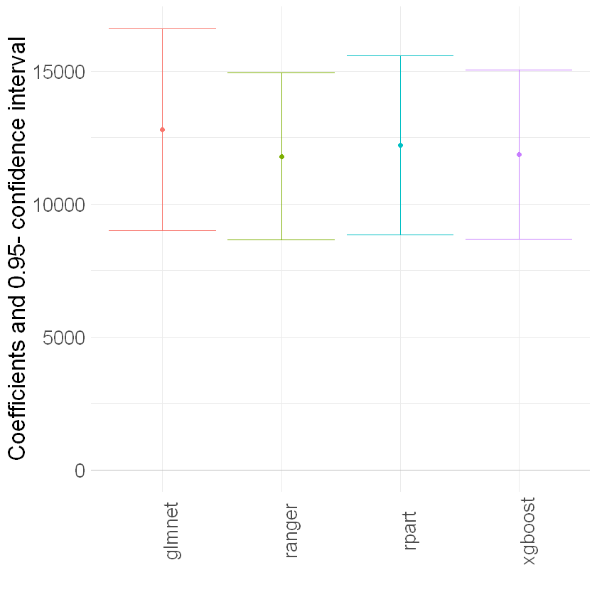
g_ci = ggplot(result_iivm, aes(x = ML, y = Estimate, color = ML)) +
        geom_point() +
        geom_errorbar(aes(ymin = lower, ymax = upper, color = ML))  +
        geom_hline(yintercept = 0, color = "grey") +
        theme_minimal() + ylab("Coefficients and 0.95- confidence interval") +
        xlab("") +
        theme(axis.text.x = element_text(angle = 90), legend.position = "none",
              text = element_text(size = 20))

g_ci

A data.table: 4 × 5

model	ML	Estimate	lower	upper
<chr>	<chr>	<dbl>	<dbl>	<dbl>
IIVM	glmnet	12802.26	8998.639	16605.88
IIVM	ranger	11792.22	8648.579	14935.87
IIVM	rpart	12214.45	8855.864	15573.04
IIVM	xgboost	11861.19	8687.158	15035.22

Summary of Results

To sum up, let’s merge all our results so far and illustrate them in a plot.

summary_result = rbindlist(list(result_plr, result_irm, result_iivm))
summary_result[, model := factor(model, levels = c("PLR", "IRM", "IIVM"))]

g_all = ggplot(summary_result, aes(x = ML, y = Estimate, color = ML)) +
        geom_point() +
        geom_errorbar(aes(ymin = lower, ymax = upper, color = ML))  +
        geom_hline(yintercept = 0, color = "grey") +
        theme_minimal() + ylab("Coefficients and 0.95- confidence interval") +
        xlab("") +
        theme(axis.text.x = element_text(angle = 90), legend.position = "none",
              text = element_text(size = 20)) +
        facet_wrap(model ~., ncol = 1)

g_all

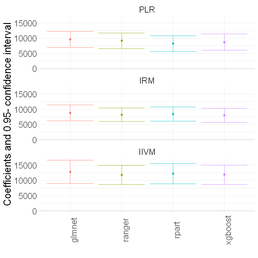
We report results based on four ML methods for estimating the nuisance functions used in forming the orthogonal estimating equations. We find again that the estimates of the treatment effect are stable across ML methods. The estimates are highly significant, hence we would reject the hypothesis that 401(k) participation has no effect on financial wealth.

---

Acknowledgement

We would like to thank Jannis Kueck for sharing the kaggle notebook. The pension data set has been analyzed in several studies, among others Chernozhukov et al. (2018).