Note
-
Download Jupyter notebook:
https://docs.doubleml.org/stable/examples/did/py_panel_simple.ipynb.
Python: Panel Data Introduction#
In this example, we replicate the results from the guide Getting Started with the did Package of the did-R-package.
As the did-R-package the implementation of DoubleML is based on Callaway and Sant’Anna(2021).
The notebook requires the following packages:
[1]:
import pandas as pd
import numpy as np

from sklearn.linear_model import LinearRegression, LogisticRegression

from doubleml.data import DoubleMLPanelData
from doubleml.did import DoubleMLDIDMulti
Data#
The data we will use is simulated and part of the CSDID-Python-Package.
A description of the data generating process can be found at the CSDID-documentation.
[2]:
dta = pd.read_csv("https://raw.githubusercontent.com/d2cml-ai/csdid/main/data/sim_data.csv")
dta.head()
[2]:
| G | X | id | cluster | period | Y | treat | |
|---|---|---|---|---|---|---|---|
| 0 | 3 | -0.876233 | 1 | 5 | 1 | 5.562556 | 1 |
| 1 | 3 | -0.876233 | 1 | 5 | 2 | 4.349213 | 1 |
| 2 | 3 | -0.876233 | 1 | 5 | 3 | 7.134037 | 1 |
| 3 | 3 | -0.876233 | 1 | 5 | 4 | 6.243056 | 1 |
| 4 | 2 | -0.873848 | 2 | 36 | 1 | -3.659387 | 1 |
To work with the DoubleML-package, we initialize a DoubleMLPanelData object.
Therefore, we set the never-treated units in group column G to np.inf (we have to change the datatype to float).
[3]:
# set dtype for G to float
dta["G"] = dta["G"].astype(float)
dta.loc[dta["G"] == 0, "G"] = np.inf
dta.head()
[3]:
| G | X | id | cluster | period | Y | treat | |
|---|---|---|---|---|---|---|---|
| 0 | 3.0 | -0.876233 | 1 | 5 | 1 | 5.562556 | 1 |
| 1 | 3.0 | -0.876233 | 1 | 5 | 2 | 4.349213 | 1 |
| 2 | 3.0 | -0.876233 | 1 | 5 | 3 | 7.134037 | 1 |
| 3 | 3.0 | -0.876233 | 1 | 5 | 4 | 6.243056 | 1 |
| 4 | 2.0 | -0.873848 | 2 | 36 | 1 | -3.659387 | 1 |
Now, we can initialize the DoubleMLPanelData object, specifying
y_col: the outcomed_cols: the group variable indicating the first treated period for each unitid_col: the unique identification column for each unitt_col: the time columnx_cols: the additional pre-treatment controls
[4]:
dml_data = DoubleMLPanelData(
    data=dta,
    y_col="Y",
    d_cols="G",
    id_col="id",
    t_col="period",
    x_cols=["X"]
)
print(dml_data)
================== DoubleMLPanelData Object ==================

------------------ Data summary      ------------------
Outcome variable: Y
Treatment variable(s): ['G']
Covariates: ['X']
Instrument variable(s): None
Time variable: period
Id variable: id
Static panel data: False
No. Unique Ids: 3979
No. Observations: 15916
------------------ DataFrame info    ------------------
<class 'pandas.DataFrame'>
RangeIndex: 15916 entries, 0 to 15915
Columns: 7 entries, G to treat
dtypes: float64(3), int64(4)
memory usage: 870.5 KB
ATT Estimation#
The DoubleML-package implements estimation of group-time average treatment effect via the DoubleMLDIDMulti class (see model documentation).
The class basically behaves like other DoubleML classes and requires the specification of two learners (for more details on the regression elements, see score documentation). The model will be estimated using the fit() method.
[5]:
dml_obj = DoubleMLDIDMulti(
    obj_dml_data=dml_data,
    ml_g=LinearRegression(),
    ml_m=LogisticRegression(),
    control_group="never_treated",
)

dml_obj.fit()
print(dml_obj)
================== DoubleMLDIDMulti Object ==================

------------------ Data summary      ------------------
Outcome variable: Y
Treatment variable(s): ['G']
Covariates: ['X']
Instrument variable(s): None
Time variable: period
Id variable: id
Static panel data: False
No. Unique Ids: 3979
No. Observations: 15916
------------------ Score & algorithm ------------------
Score function: observational
Control group: never_treated
Anticipation periods: 0

------------------ Machine learner   ------------------
Learner ml_g: LinearRegression()
Learner ml_m: LogisticRegression()
Out-of-sample Performance:
Regression:
Learner ml_g0 RMSE: [[1.42556994 1.41127551 1.39871895 1.42551492 1.40900895 1.42030423
  1.42565583 1.40606521 1.42885737]]
Learner ml_g1 RMSE: [[1.40278936 1.43916139 1.39656991 1.41565792 1.4265632  1.38457948
  1.45647481 1.41776112 1.40829183]]
Classification:
Learner ml_m Log Loss: [[0.69093517 0.69099994 0.69049595 0.67910089 0.67952164 0.68058919
  0.66204308 0.66226317 0.66256381]]

------------------ Resampling        ------------------
No. folds: 5
No. repeated sample splits: 1

------------------ Fit summary       ------------------
                  coef   std err          t     P>|t|     2.5 %    97.5 %
ATT(2.0,1,2)  0.923651  0.063989  14.434481  0.000000  0.798235  1.049068
ATT(2.0,1,3)  1.985174  0.064661  30.701089  0.000000  1.858440  2.111908
ATT(2.0,1,4)  2.954626  0.063164  46.776820  0.000000  2.830827  3.078426
ATT(3.0,1,2) -0.042314  0.065921  -0.641883  0.520949 -0.171516  0.086889
ATT(3.0,2,3)  1.110035  0.065501  16.946814  0.000000  0.981655  1.238415
ATT(3.0,2,4)  2.062428  0.065553  31.461797  0.000000  1.933946  2.190911
ATT(4.0,1,2)  0.003296  0.068525   0.048096  0.961640 -0.131011  0.137602
ATT(4.0,2,3)  0.061200  0.066547   0.919641  0.357760 -0.069231  0.191630
ATT(4.0,3,4)  0.962677  0.067883  14.181395  0.000000  0.829628  1.095725
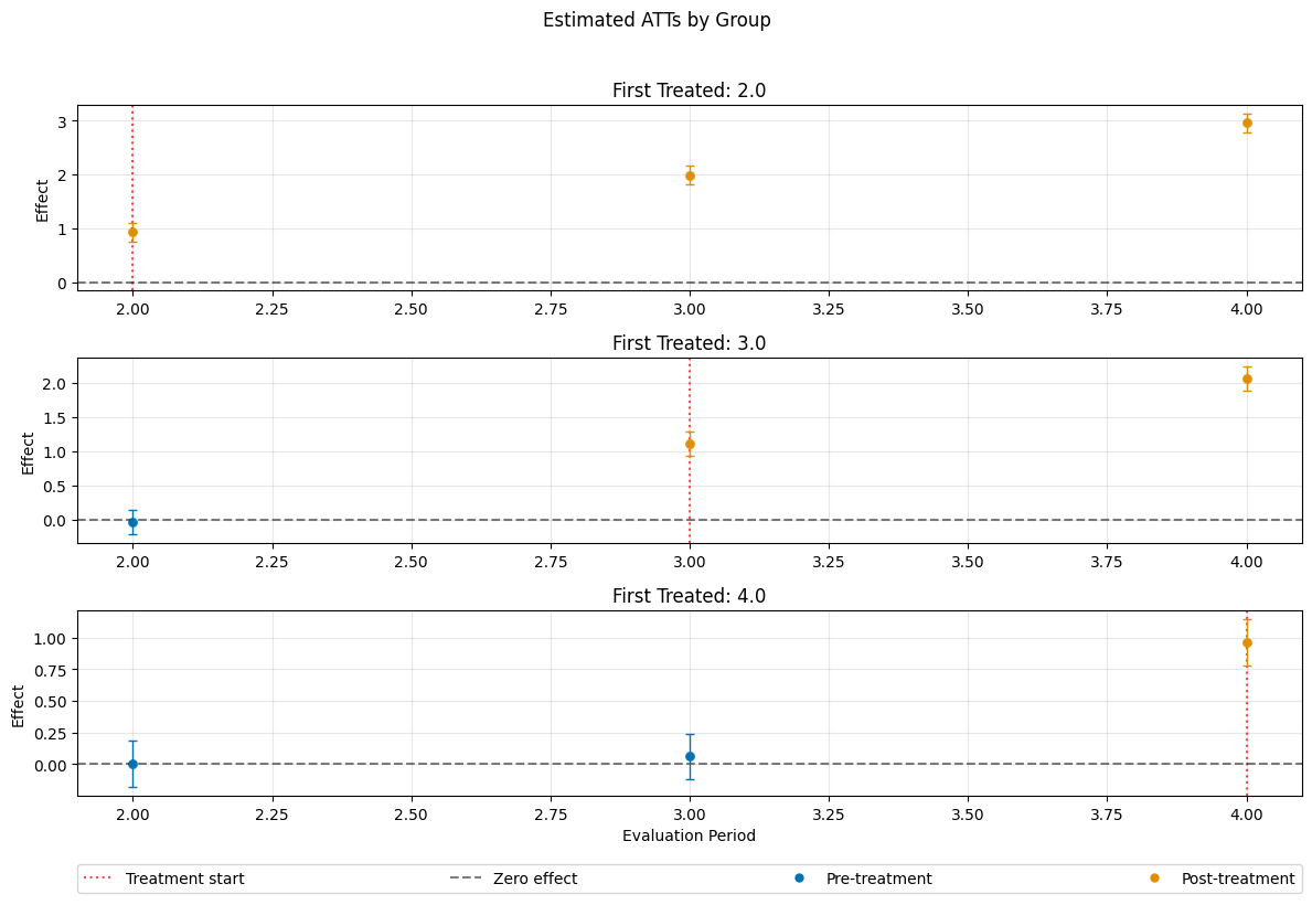
The summary displays estimates of the \(ATT(g,t_\text{eval})\) effects for different combinations of \((g,t_\text{eval})\) via \(\widehat{ATT}(\mathrm{g},t_\text{pre},t_\text{eval})\), where
\(\mathrm{g}\) specifies the group
\(t_\text{pre}\) specifies the corresponding pre-treatment period
\(t_\text{eval}\) specifies the evaluation period
This corresponds to the estimates given in att_gt function in the did-R-package, where the standard choice is \(t_\text{pre} = \min(\mathrm{g}, t_\text{eval}) - 1\) (without anticipation).
Remark that this includes pre-tests effects if \(\mathrm{g} > t_{eval}\), e.g. \(ATT(4,2)\).
As usual for the DoubleML-package, you can obtain joint confidence intervals via bootstrap.
[6]:
level = 0.95

ci = dml_obj.confint(level=level)
dml_obj.bootstrap(n_rep_boot=5000)
ci_joint = dml_obj.confint(level=level, joint=True)
ci_joint
[6]:
| 2.5 % | 97.5 % | |
|---|---|---|
| ATT(2.0,1,2) | 0.750542 | 1.096760 |
| ATT(2.0,1,3) | 1.810246 | 2.160101 |
| ATT(2.0,1,4) | 2.783749 | 3.125504 |
| ATT(3.0,1,2) | -0.220648 | 0.136021 |
| ATT(3.0,2,3) | 0.932836 | 1.287235 |
| ATT(3.0,2,4) | 1.885088 | 2.239769 |
| ATT(4.0,1,2) | -0.182084 | 0.188676 |
| ATT(4.0,2,3) | -0.118830 | 0.241230 |
| ATT(4.0,3,4) | 0.779034 | 1.146320 |
A visualization of the effects can be obtained via the plot_effects() method.
Remark that the plot used joint confidence intervals per default.
[7]:
fig, ax = dml_obj.plot_effects()
Effect Aggregation#
As the did-R-package, the \(ATT\)’s can be aggregated to summarize multiple effects. For details on different aggregations and details on their interpretations see Callaway and Sant’Anna(2021).
The aggregations are implemented via the aggregate() method.
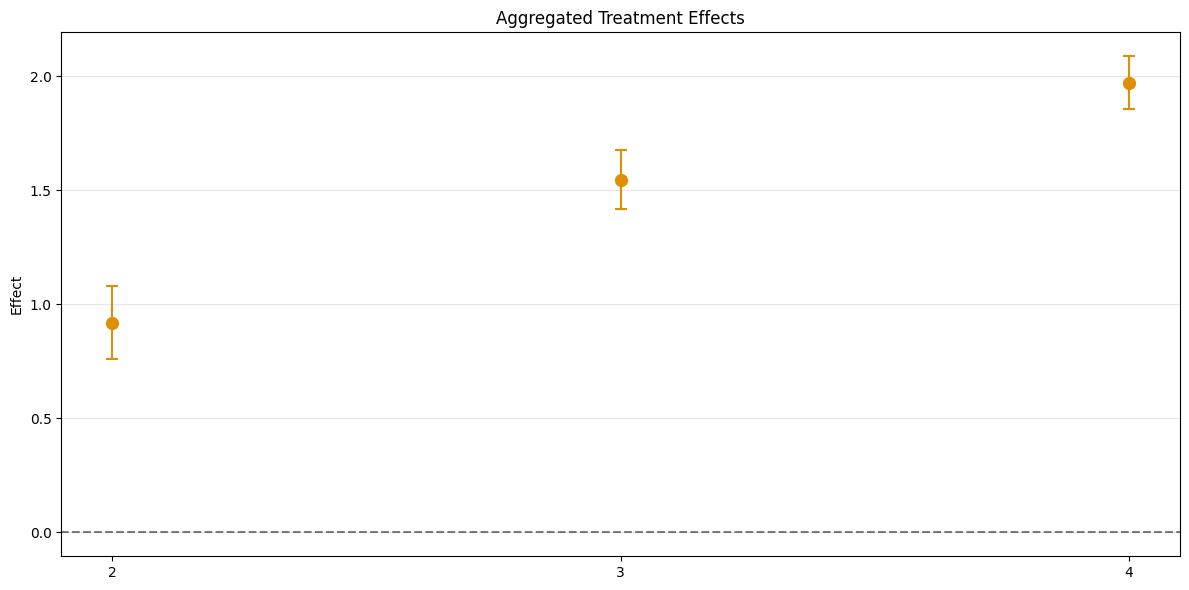
Group Aggregation#
To obtain group-specific effects it is possible to aggregate several \(\widehat{ATT}(\mathrm{g},t_\text{pre},t_\text{eval})\) values based on the group \(\mathrm{g}\) by setting the aggregation="group" argument.
[8]:
aggregated = dml_obj.aggregate(aggregation="group")
print(aggregated)
_ = aggregated.plot_effects()
================== DoubleMLDIDAggregation Object ==================
 Group Aggregation

------------------ Overall Aggregated Effects ------------------
    coef  std err         t  P>|t|    2.5 %   97.5 %
1.492479 0.034344 43.456834    0.0 1.425166 1.559792
------------------ Aggregated Effects         ------------------
         coef   std err          t  P>|t|     2.5 %    97.5 %
2.0  1.954484  0.052227  37.423077    0.0  1.852121  2.056846
3.0  1.586232  0.056313  28.167918    0.0  1.475860  1.696604
4.0  0.962677  0.067883  14.181395    0.0  0.829628  1.095725
------------------ Additional Information     ------------------
Score function: observational
Control group: never_treated
Anticipation periods: 0
/opt/hostedtoolcache/Python/3.12.13/x64/lib/python3.12/site-packages/doubleml/did/did_aggregation.py:368: UserWarning: Joint confidence intervals require bootstrapping which hasn't been performed yet. Automatically applying '.aggregated_frameworks.bootstrap(method="normal", n_rep_boot=500)' with default values. For different bootstrap settings, call bootstrap() explicitly before plotting.
  warnings.warn(
The output is a DoubleMLDIDAggregation object which includes an overall aggregation summary based on group size.
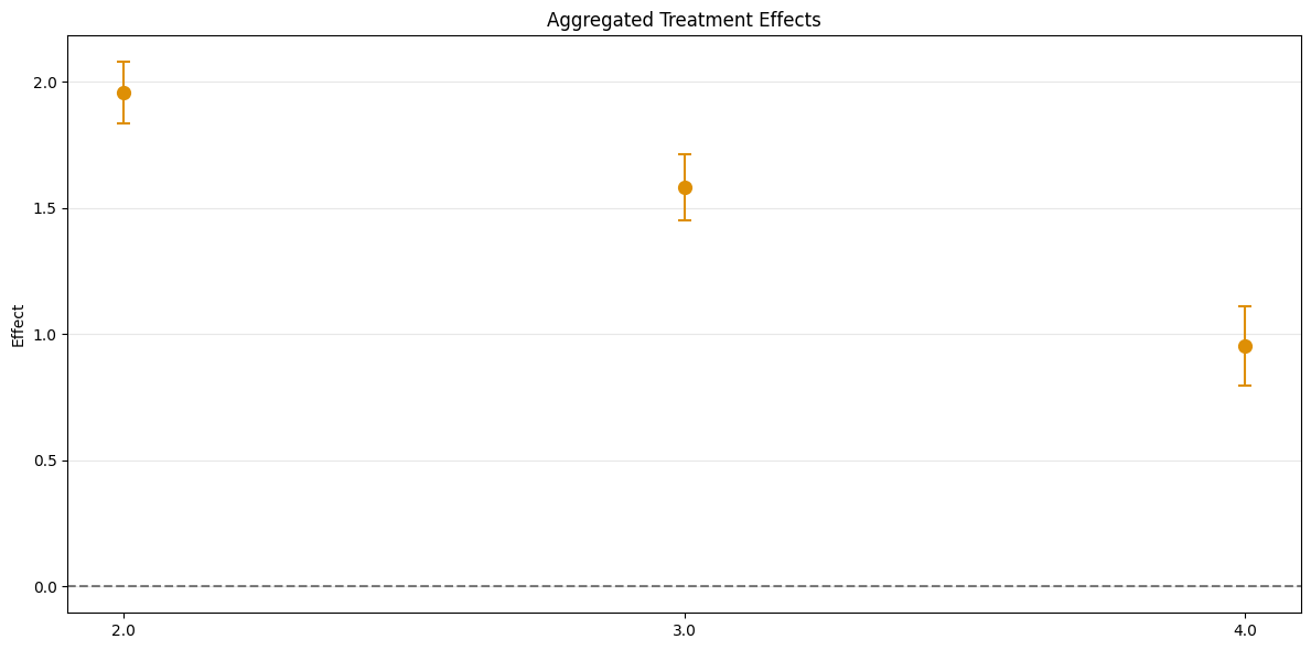
Time Aggregation#
This aggregates \(\widehat{ATT}(\mathrm{g},t_\text{pre},t_\text{eval})\), based on \(t_\text{eval}\), but weighted with respect to group size. Corresponds to Calendar Time Effects from the did-R-package.
For calendar time effects set aggregation="time".
[9]:
aggregated_time = dml_obj.aggregate("time")
print(aggregated_time)
fig, ax = aggregated_time.plot_effects()
================== DoubleMLDIDAggregation Object ==================
 Time Aggregation

------------------ Overall Aggregated Effects ------------------
    coef  std err         t  P>|t|    2.5 %   97.5 %
1.483157 0.035103 42.251971    0.0 1.414357 1.551957
------------------ Aggregated Effects         ------------------
       coef   std err          t  P>|t|     2.5 %    97.5 %
2  0.923651  0.063989  14.434481    0.0  0.798235  1.049068
3  1.548947  0.051392  30.139565    0.0  1.448219  1.649674
4  1.976873  0.046736  42.298858    0.0  1.885272  2.068473
------------------ Additional Information     ------------------
Score function: observational
Control group: never_treated
Anticipation periods: 0
/opt/hostedtoolcache/Python/3.12.13/x64/lib/python3.12/site-packages/doubleml/did/did_aggregation.py:368: UserWarning: Joint confidence intervals require bootstrapping which hasn't been performed yet. Automatically applying '.aggregated_frameworks.bootstrap(method="normal", n_rep_boot=500)' with default values. For different bootstrap settings, call bootstrap() explicitly before plotting.
  warnings.warn(
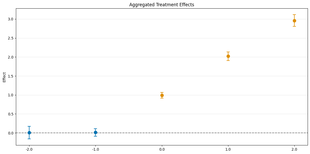
Event Study Aggregation#
Finally, aggregation="eventstudy" aggregates \(\widehat{ATT}(\mathrm{g},t_\text{pre},t_\text{eval})\) based on exposure time \(e = t_\text{eval} - \mathrm{g}\) (respecting group size).
[10]:
aggregated_eventstudy = dml_obj.aggregate("eventstudy")
print(aggregated_eventstudy)
fig, ax = aggregated_eventstudy.plot_effects()
================== DoubleMLDIDAggregation Object ==================
 Event Study Aggregation

------------------ Overall Aggregated Effects ------------------
    coef  std err         t  P>|t|    2.5 %   97.5 %
1.992101 0.038748 51.411397    0.0 1.916156 2.068047
------------------ Aggregated Effects         ------------------
          coef   std err          t     P>|t|     2.5 %    97.5 %
-2.0  0.003296  0.068525   0.048096  0.961640 -0.131011  0.137602
-1.0  0.010813  0.040541   0.266705  0.789696 -0.068647  0.090272
0.0   0.997995  0.030809  32.393358  0.000000  0.937612  1.058379
1.0   2.023683  0.045701  44.280625  0.000000  1.934110  2.113255
2.0   2.954626  0.063164  46.776820  0.000000  2.830827  3.078426
------------------ Additional Information     ------------------
Score function: observational
Control group: never_treated
Anticipation periods: 0
/opt/hostedtoolcache/Python/3.12.13/x64/lib/python3.12/site-packages/doubleml/did/did_aggregation.py:368: UserWarning: Joint confidence intervals require bootstrapping which hasn't been performed yet. Automatically applying '.aggregated_frameworks.bootstrap(method="normal", n_rep_boot=500)' with default values. For different bootstrap settings, call bootstrap() explicitly before plotting.
  warnings.warn(
Aggregation Details#
The DoubleMLDIDAggregation objects include several DoubleMLFrameworks which support methods like bootstrap() or confint(). Further, the weights can be accessed via the properties
overall_aggregation_weights: weights for the overall aggregationaggregation_weights: weights for the aggregation
To clarify, e.g. for the eventstudy aggregation
[11]:
print(aggregated_eventstudy)
================== DoubleMLDIDAggregation Object ==================
 Event Study Aggregation

------------------ Overall Aggregated Effects ------------------
    coef  std err         t  P>|t|    2.5 %   97.5 %
1.992101 0.038748 51.411397    0.0 1.916156 2.068047
------------------ Aggregated Effects         ------------------
          coef   std err          t     P>|t|     2.5 %    97.5 %
-2.0  0.003296  0.068525   0.048096  0.961640 -0.131011  0.137602
-1.0  0.010813  0.040541   0.266705  0.789696 -0.068647  0.090272
0.0   0.997995  0.030809  32.393358  0.000000  0.937612  1.058379
1.0   2.023683  0.045701  44.280625  0.000000  1.934110  2.113255
2.0   2.954626  0.063164  46.776820  0.000000  2.830827  3.078426
------------------ Additional Information     ------------------
Score function: observational
Control group: never_treated
Anticipation periods: 0
Here, the overall effect aggregation aggregates each effect with positive exposure
[12]:
print(aggregated_eventstudy.overall_aggregation_weights)
[0. 0. 0.33333333 0.33333333 0.33333333]
If one would like to consider how the aggregated effect with \(e=0\) is computed, one would have to look at the third set of weights within the aggregation_weights property
[13]:
aggregated_eventstudy.aggregation_weights[2]
[13]:
array([0.32875335, 0.        , 0.        , 0.        , 0.32674263,
       0.        , 0.        , 0.        , 0.34450402])
Taking a look at the original dml_obj, one can see that this combines the following estimates:
\(\widehat{ATT}(2,1,2)\)
\(\widehat{ATT}(3,2,3)\)
\(\widehat{ATT}(4,3,4)\)
[14]:
print(dml_obj.summary)
                  coef   std err          t     P>|t|     2.5 %    97.5 %
ATT(2.0,1,2)  0.923651  0.063989  14.434481  0.000000  0.798235  1.049068
ATT(2.0,1,3)  1.985174  0.064661  30.701089  0.000000  1.858440  2.111908
ATT(2.0,1,4)  2.954626  0.063164  46.776820  0.000000  2.830827  3.078426
ATT(3.0,1,2) -0.042314  0.065921  -0.641883  0.520949 -0.171516  0.086889
ATT(3.0,2,3)  1.110035  0.065501  16.946814  0.000000  0.981655  1.238415
ATT(3.0,2,4)  2.062428  0.065553  31.461797  0.000000  1.933946  2.190911
ATT(4.0,1,2)  0.003296  0.068525   0.048096  0.961640 -0.131011  0.137602
ATT(4.0,2,3)  0.061200  0.066547   0.919641  0.357760 -0.069231  0.191630
ATT(4.0,3,4)  0.962677  0.067883  14.181395  0.000000  0.829628  1.095725