Note

Download Jupyter notebook: https://docs.doubleml.org/stable/examples/py_double_ml_basics.ipynb.

Python: Basics of Double Machine Learning

Remark: This notebook has a long computation time due to the large number of simulations.

This notebooks contains the detailed simulations according to the introduction to double machine learning in the User Guide of the DoubleML package.

import warnings
import numpy as np
from scipy import stats
import matplotlib.pyplot as plt
import seaborn as sns

from lightgbm import LGBMRegressor
from sklearn.ensemble import RandomForestRegressor
from sklearn.model_selection import train_test_split
from sklearn.base import clone

from doubleml import DoubleMLData
from doubleml import DoubleMLPLR
from doubleml.datasets import make_plr_CCDDHNR2018

face_colors = sns.color_palette('pastel')
edge_colors = sns.color_palette('dark')

warnings.filterwarnings("ignore")

Data Generating Process (DGP)

We consider the following partially linear model:

\[\begin{split}\begin{align*} y_i &= \theta_0 d_i + g_0(x_i) + \zeta_i, & \zeta_i \sim \mathcal{N}(0,1), \\ d_i &= m_0(x_i) + v_i, & v_i \sim \mathcal{N}(0,1), \end{align*}\end{split}\]

with covariates \(x_i \sim \mathcal{N}(0, \Sigma)\), where \(\Sigma\) is a matrix with entries \(\Sigma_{kj} = 0.7^{|j-k|}\). We are interested in performing valid inference on the causal parameter \(\theta_0\). The true parameter \(\theta_0\) is set to \(0.5\) in our simulation experiment.

The nuisance functions are given by:

\[\begin{split}\begin{align*} m_0(x_i) &= x_{i,1} + \frac{1}{4} \frac{\exp(x_{i,3})}{1+\exp(x_{i,3})}, \\ g_0(x_i) &= \frac{\exp(x_{i,1})}{1+\exp(x_{i,1})} + \frac{1}{4} x_{i,3}. \end{align*}\end{split}\]

We generate n_rep replications of the data generating process with sample size n_obs and compare the performance of different estimators.

np.random.seed(1234)
n_rep = 1000
n_obs = 500
n_vars = 5
alpha = 0.5

data = list()

for i_rep in range(n_rep):
    (x, y, d) = make_plr_CCDDHNR2018(alpha=alpha, n_obs=n_obs, dim_x=n_vars, return_type='array')
    data.append((x, y, d))

Regularization Bias in Simple ML-Approaches

Naive inference that is based on a direct application of machine learning methods to estimate the causal parameter, \(\theta_0\), is generally invalid. The use of machine learning methods introduces a bias that arises due to regularization. A simple ML approach is given by randomly splitting the sample into two parts. On the auxiliary sample indexed by \(i \in I^C\) the nuisance function \(g_0(X)\) is estimated with an ML method, for example a random forest learner. Given the estimate \(\hat{g}_0(X)\), the final estimate of \(\theta_0\) is obtained as (\(n=N/2\)) using the other half of observations indexed with \(i \in I\)

\[\hat{\theta}_0 = \left(\frac{1}{n} \sum_{i\in I} D_i^2\right)^{-1} \frac{1}{n} \sum_{i\in I} D_i (Y_i - \hat{g}_0(X_i)).\]

As this corresponds to a “non-orthogonal” score, which is not implemented in the DoubleML package, we need to define a custom callable.

def non_orth_score(y, d, l_hat, m_hat, g_hat, smpls):
    u_hat = y - g_hat
    psi_a = -np.multiply(d, d)
    psi_b = np.multiply(d, u_hat)
    return psi_a, psi_b

Remark that the estimator is not able to estimate \(\hat{g}_0(X)\) directly, but has to be based on a preliminary estimate of \(\hat{m}_0(X)\). All following estimators with score="IV-type" are based on the same preliminary procedure. Furthermore, remark that we are using external predictions to avoid cross-fitting (for demonstration purposes).

np.random.seed(1111)

ml_l = LGBMRegressor(n_estimators=300, learning_rate=0.1)
ml_m = LGBMRegressor(n_estimators=300, learning_rate=0.1)
ml_l = RandomForestRegressor(n_estimators=100, max_features=10, max_depth=5, min_samples_leaf=5)
ml_m = RandomForestRegressor(n_estimators=200, max_features=10, max_depth=5, min_samples_leaf=5)

ml_g = clone(ml_l)

theta_nonorth = np.full(n_rep, np.nan)
se_nonorth = np.full(n_rep, np.nan)

for i_rep in range(n_rep):
    print(f'Replication {i_rep+1}/{n_rep}', end='\r')
    (x, y, d) = data[i_rep]

    # choose a random sample for training and estimation
    i_train, i_est = train_test_split(np.arange(n_obs), test_size=0.5, random_state=42)

    # fit the ML algorithms on the training sample
    ml_l.fit(x[i_train, :], y[i_train])
    ml_m.fit(x[i_train, :], d[i_train])

    psi_a = -np.multiply(d[i_train] - ml_m.predict(x[i_train, :]), d[i_train] - ml_m.predict(x[i_train, :]))
    psi_b = np.multiply(d[i_train] - ml_m.predict(x[i_train, :]), y[i_train] - ml_l.predict(x[i_train, :]))
    theta_initial = -np.nanmean(psi_b) / np.nanmean(psi_a)
    ml_g.fit(x[i_train, :], y[i_train] - theta_initial * d[i_train])

    # create out-of-sample predictions
    l_hat = ml_l.predict(x[i_est, :])
    m_hat = ml_m.predict(x[i_est, :])
    g_hat = ml_g.predict(x[i_est, :])

    external_predictions = {
        'd': {
            'ml_l': l_hat.reshape(-1, 1),
            'ml_m': m_hat.reshape(-1, 1),
            'ml_g': g_hat.reshape(-1, 1)
        }
    }

    obj_dml_data = DoubleMLData.from_arrays(x[i_est, :], y[i_est], d[i_est])
    obj_dml_plr_nonorth = DoubleMLPLR(obj_dml_data,
                                    ml_l, ml_m, ml_g,
                                    n_folds=2,
                                    score=non_orth_score)
    obj_dml_plr_nonorth.fit(external_predictions=external_predictions)
    theta_nonorth[i_rep] = obj_dml_plr_nonorth.coef[0]
    se_nonorth[i_rep] = obj_dml_plr_nonorth.se[0]

fig_non_orth, ax = plt.subplots(constrained_layout=True);
ax = sns.histplot((theta_nonorth - alpha)/se_nonorth,
                color=face_colors[0], edgecolor = edge_colors[0],
                stat='density', bins=30, label='Non-orthogonal ML');
ax.axvline(0., color='k');
xx = np.arange(-5, +5, 0.001)
yy = stats.norm.pdf(xx)
ax.plot(xx, yy, color='k', label='$\\mathcal{N}(0, 1)$');
ax.legend(loc='upper right', bbox_to_anchor=(1.2, 1.0));
ax.set_xlim([-6., 6.]);
ax.set_xlabel('$(\hat{\\theta}_0 - \\theta_0)/\hat{\sigma}$');
plt.show()

Replication 1000/1000

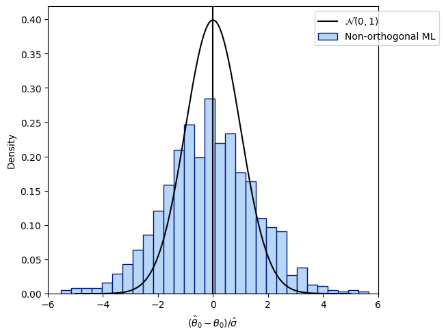
The regularization bias in the simple ML-approach is caused by the slow convergence of \(\hat{\theta}_0\)

\[|\sqrt{n} (\hat{\theta}_0 - \theta_0) | \rightarrow_{P} \infty\]

i.e., slower than \(1/\sqrt{n}\). The driving factor is the bias that arises by learning \(g\) with a random forest or any other ML technique. A heuristic illustration is given by

\[\sqrt{n}(\hat{\theta}_0 - \theta_0) = \underbrace{\left(\frac{1}{n} \sum_{i\in I} D_i^2\right)^{-1} \frac{1}{n} \sum_{i\in I} D_i \zeta_i}_{=:a} + \underbrace{\left(\frac{1}{n} \sum_{i\in I} D_i^2\right)^{-1} \frac{1}{n} \sum_{i\in I} D_i (g_0(X_i) - \hat{g}_0(X_i))}_{=:b}.\]

\(a\) is approximately Gaussian under mild conditions. However, \(b\) (the regularization bias) diverges in general.

Overcoming regularization bias by orthogonalization

To overcome the regularization bias we can partial out the effect of \(X\) from \(D\) to obtain the orthogonalized regressor \(V = D - m(X)\). We then use the final estimate

\[\check{\theta}_0 = \left(\frac{1}{n} \sum_{i\in I} \hat{V}_i D_i\right)^{-1} \frac{1}{n} \sum_{i\in I} \hat{V}_i (Y_i - \hat{g}_0(X_i)).\]

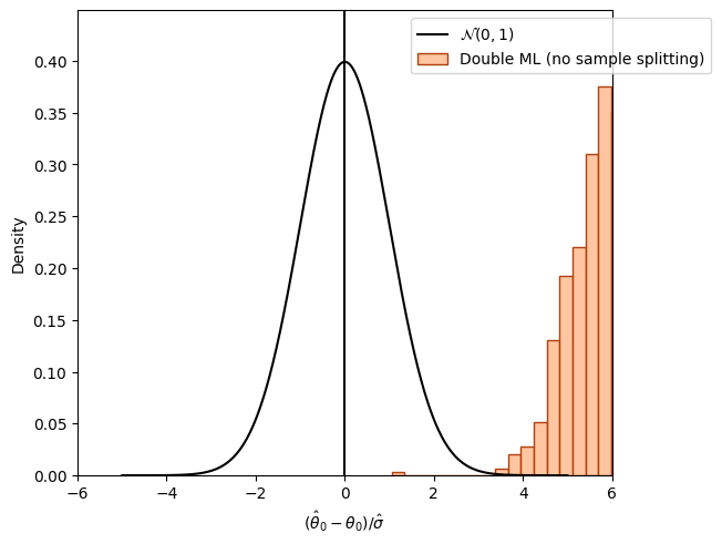
The following figure shows the distribution of the resulting estimates \(\hat{\theta}_0\) without sample-splitting. Again, we are using external predictions to avoid cross-fitting (for demonstration purposes).

np.random.seed(2222)

theta_orth_nosplit = np.full(n_rep, np.nan)
se_orth_nosplit = np.full(n_rep, np.nan)

for i_rep in range(n_rep):
    print(f'Replication {i_rep+1}/{n_rep}', end='\r')
    (x, y, d) = data[i_rep]

    # fit the ML algorithms on the training sample
    ml_l.fit(x, y)
    ml_m.fit(x, d)

    psi_a = -np.multiply(d - ml_m.predict(x), d - ml_m.predict(x))
    psi_b = np.multiply(d - ml_m.predict(x), y - ml_l.predict(x))
    theta_initial = -np.nanmean(psi_b) / np.nanmean(psi_a)
    ml_g.fit(x, y - theta_initial * d)

    l_hat = ml_l.predict(x)
    m_hat = ml_m.predict(x)
    g_hat = ml_g.predict(x)

    external_predictions = {
        'd': {
            'ml_l': l_hat.reshape(-1, 1),
            'ml_m': m_hat.reshape(-1, 1),
            'ml_g': g_hat.reshape(-1, 1)
        }
    }

    obj_dml_data = DoubleMLData.from_arrays(x, y, d)

    obj_dml_plr_orth_nosplit = DoubleMLPLR(obj_dml_data,
                                        ml_l, ml_m, ml_g,
                                        score='IV-type')
    obj_dml_plr_orth_nosplit.fit(external_predictions=external_predictions)
    theta_orth_nosplit[i_rep] = obj_dml_plr_orth_nosplit.coef[0]
    se_orth_nosplit[i_rep] = obj_dml_plr_orth_nosplit.se[0]

fig_orth_nosplit, ax = plt.subplots(constrained_layout=True);
ax = sns.histplot((theta_orth_nosplit - alpha)/se_orth_nosplit,
                color=face_colors[1], edgecolor = edge_colors[1],
                stat='density', bins=30, label='Double ML (no sample splitting)');
ax.axvline(0., color='k');
xx = np.arange(-5, +5, 0.001)
yy = stats.norm.pdf(xx)
ax.plot(xx, yy, color='k', label='$\\mathcal{N}(0, 1)$');
ax.legend(loc='upper right', bbox_to_anchor=(1.2, 1.0));
ax.set_xlim([-6., 6.]);
ax.set_xlabel('$(\hat{\\theta}_0 - \\theta_0)/\hat{\sigma}$');
plt.show()

Replication 1000/1000

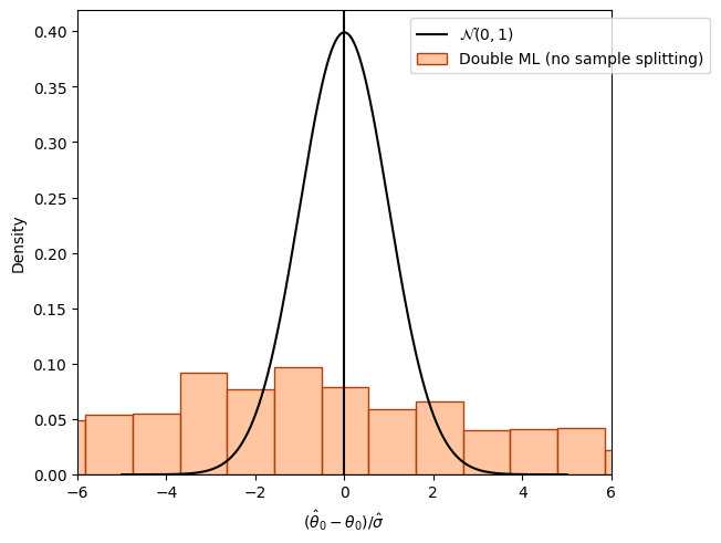
If the nuisance models \(\hat{g}_0()\) and \(\hat{m}()\) are estimated on the whole dataset, which is also used for obtaining the final estimate \(\check{\theta}_0\), another bias is observed.

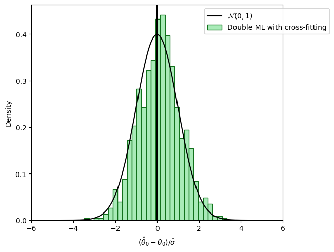
Sample splitting to remove bias induced by overfitting

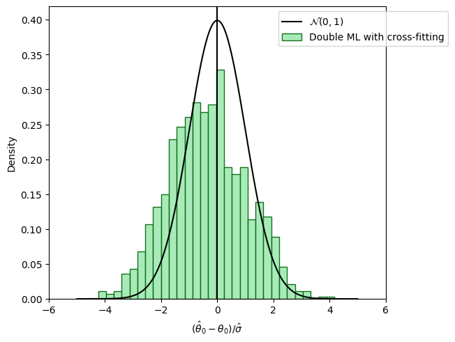
Using sample splitting, i.e., estimate the nuisance models \(\hat{g}_0()\) and \(\hat{m}()\) on one part of the data (training data) and estimate \(\check{\theta}_0\) on the other part of the data (test data), overcomes the bias induced by overfitting. We can exploit the benefits of cross-fitting by switching the role of the training and test sample. Cross-fitting performs well empirically because the entire sample can be used for estimation.

The following figure shows the distribution of the resulting estimates \(\hat{\theta}_0\) with orthogonal score and sample-splitting.

np.random.seed(3333)

theta_dml = np.full(n_rep, np.nan)
se_dml = np.full(n_rep, np.nan)

for i_rep in range(n_rep):
    print(f'Replication {i_rep+1}/{n_rep}', end='\r')
    (x, y, d) = data[i_rep]
    obj_dml_data = DoubleMLData.from_arrays(x, y, d)
    obj_dml_plr = DoubleMLPLR(obj_dml_data,
                            ml_l, ml_m, ml_g,
                            n_folds=2,
                            score='IV-type')
    obj_dml_plr.fit()
    theta_dml[i_rep] = obj_dml_plr.coef[0]
    se_dml[i_rep] = obj_dml_plr.se[0]

fig_dml, ax = plt.subplots(constrained_layout=True);
ax = sns.histplot((theta_dml - alpha)/se_dml,
                color=face_colors[2], edgecolor = edge_colors[2],
                stat='density', bins=30, label='Double ML with cross-fitting');
ax.axvline(0., color='k');
xx = np.arange(-5, +5, 0.001)
yy = stats.norm.pdf(xx)
ax.plot(xx, yy, color='k', label='$\\mathcal{N}(0, 1)$');
ax.legend(loc='upper right', bbox_to_anchor=(1.2, 1.0));
ax.set_xlim([-6., 6.]);
ax.set_xlabel('$(\hat{\\theta}_0 - \\theta_0)/\hat{\sigma}$');
plt.show()

Replication 1000/1000

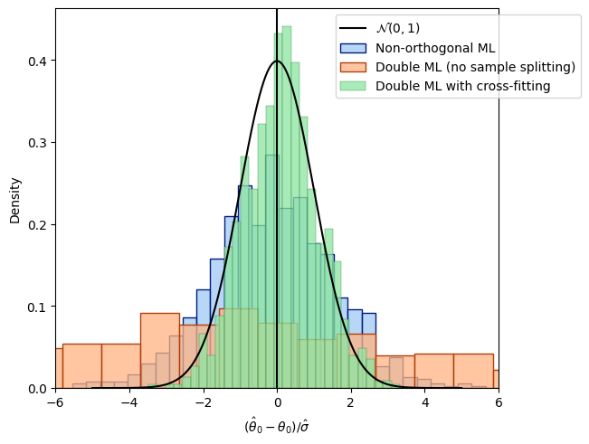
Double/debiased machine learning

To illustrate the benefits of the auxiliary prediction step in the DML framework we write the error as

\[\sqrt{n}(\check{\theta}_0 - \theta_0) = a^* + b^* + c^*\]

Chernozhukov et al. (2018) argues that:

The first term

\[a^* := (EV^2)^{-1} \frac{1}{\sqrt{n}} \sum_{i\in I} V_i \zeta_i\]

will be asymptotically normally distributed.

The second term

\[b^* := (EV^2)^{-1} \frac{1}{\sqrt{n}} \sum_{i\in I} (\hat{m}(X_i) - m(X_i)) (\hat{g}_0(X_i) - g_0(X_i))\]

vanishes asymptotically for many data generating processes.

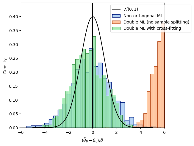
The third term \(c^*\) vanishes in probability if sample splitting is applied. Finally, let us compare all distributions.

fig_all, ax = plt.subplots(constrained_layout=True);
ax = sns.histplot((theta_nonorth - alpha)/se_nonorth,
                 color=face_colors[0], edgecolor = edge_colors[0],
                 stat='density', bins=30, label='Non-orthogonal ML');
sns.histplot((theta_orth_nosplit - alpha)/se_orth_nosplit,
             color=face_colors[1], edgecolor = edge_colors[1],
             stat='density', bins=30, label='Double ML (no sample splitting)');
sns.histplot((theta_dml - alpha)/se_dml,
             color=face_colors[2], edgecolor = edge_colors[2],
             stat='density', bins=30, label='Double ML with cross-fitting');
ax.axvline(0., color='k');
xx = np.arange(-5, +5, 0.001)
yy = stats.norm.pdf(xx)
ax.plot(xx, yy, color='k', label='$\\mathcal{N}(0, 1)$');
ax.legend(loc='upper right', bbox_to_anchor=(1.2, 1.0));
ax.set_xlim([-6., 6.]);
ax.set_xlabel('$(\hat{\\theta}_0 - \\theta_0)/\hat{\sigma}$');
plt.show()

Partialling out score

Another debiased estimator, based on the partialling-out approach of Robinson(1988), is

\[\check{\theta}_0 = \left(\frac{1}{n} \sum_{i\in I} \hat{V}_i \hat{V}_i \right)^{-1} \frac{1}{n} \sum_{i\in I} \hat{V}_i (Y_i - \hat{\ell}_0(X_i)),\]

with \(\ell_0(X_i) = E(Y|X)\). All nuisance parameters for the estimator with score='partialling out' are conditional mean functions, which can be directly estimated using ML methods. This is a minor advantage over the estimator with score='IV-type'. In the following, we repeat the above analysis with score='partialling out'. In a first part of the analysis, we estimate \(\theta_0\) without sample splitting. Again we observe a bias from overfitting.

The following figure shows the distribution of the resulting estimates \(\hat{\theta}_0\) without sample-splitting.

np.random.seed(4444)

theta_orth_po_nosplit = np.full(n_rep, np.nan)
se_orth_po_nosplit = np.full(n_rep, np.nan)

for i_rep in range(n_rep):
     print(f'Replication {i_rep+1}/{n_rep}', end='\r')
     (x, y, d) = data[i_rep]

     # fit the ML algorithms on the training sample
     ml_l.fit(x, y)
     ml_m.fit(x, d)

     l_hat = ml_l.predict(x)
     m_hat = ml_m.predict(x)

     external_predictions = {
          'd': {
               'ml_l': l_hat.reshape(-1, 1),
               'ml_m': m_hat.reshape(-1, 1),
          }
     }

     obj_dml_plr_orth_nosplit = DoubleMLPLR(obj_dml_data,
                                         ml_l, ml_m,
                                         score='partialling out')
     obj_dml_plr_orth_nosplit.fit(external_predictions=external_predictions)
     theta_orth_po_nosplit[i_rep] = obj_dml_plr_orth_nosplit.coef[0]
     se_orth_po_nosplit[i_rep] = obj_dml_plr_orth_nosplit.se[0]

fig_po_nosplit, ax = plt.subplots(constrained_layout=True);
ax = sns.histplot((theta_orth_po_nosplit - alpha)/se_orth_po_nosplit,
                 color=face_colors[1], edgecolor = edge_colors[1],
                 stat='density', bins=30, label='Double ML (no sample splitting)');
ax.axvline(0., color='k');
xx = np.arange(-5, +5, 0.001)
yy = stats.norm.pdf(xx)
ax.plot(xx, yy, color='k', label='$\\mathcal{N}(0, 1)$');
ax.legend(loc='upper right', bbox_to_anchor=(1.2, 1.0));
ax.set_xlim([-6., 6.]);
ax.set_xlabel('$(\hat{\\theta}_0 - \\theta_0)/\hat{\sigma}$');
plt.show()

Replication 1000/1000

Using sample splitting, overcomes the bias induced by overfitting. Again, the implementation automatically applies cross-fitting.

np.random.seed(5555)

theta_dml_po = np.full(n_rep, np.nan)
se_dml_po = np.full(n_rep, np.nan)

for i_rep in range(n_rep):
     print(f'Replication {i_rep+1}/{n_rep}', end='\r')
     (x, y, d) = data[i_rep]
     obj_dml_data = DoubleMLData.from_arrays(x, y, d)
     obj_dml_plr = DoubleMLPLR(obj_dml_data,
                             ml_l, ml_m,
                             n_folds=2,
                             score='partialling out')
     obj_dml_plr.fit()
     theta_dml_po[i_rep] = obj_dml_plr.coef[0]
     se_dml_po[i_rep] = obj_dml_plr.se[0]

fig_po_dml, ax = plt.subplots(constrained_layout=True);
ax = sns.histplot((theta_dml_po - alpha)/se_dml_po,
                 color=face_colors[2], edgecolor = edge_colors[2],
                 stat='density', bins=30, label='Double ML with cross-fitting');
ax.axvline(0., color='k');
xx = np.arange(-5, +5, 0.001)
yy = stats.norm.pdf(xx)
ax.plot(xx, yy, color='k', label='$\\mathcal{N}(0, 1)$');
ax.legend(loc='upper right', bbox_to_anchor=(1.2, 1.0));
ax.set_xlim([-6., 6.]);
ax.set_xlabel('$(\hat{\\theta}_0 - \\theta_0)/\hat{\sigma}$');
plt.show()

Replication 1000/1000

Finally, let us compare all distributions.

fig_po_all, ax = plt.subplots(constrained_layout=True);
ax = sns.histplot((theta_nonorth - alpha)/se_nonorth,
                color=face_colors[0], edgecolor = edge_colors[0],
                stat='density', bins=30, label='Non-orthogonal ML');
sns.histplot((theta_orth_po_nosplit - alpha)/se_orth_po_nosplit,
            color=face_colors[1], edgecolor = edge_colors[1],
            stat='density', bins=30, label='Double ML (no sample splitting)');
sns.histplot((theta_dml_po - alpha)/se_dml_po,
            color=face_colors[2], edgecolor = edge_colors[2],
            stat='density', bins=30, label='Double ML with cross-fitting');
ax.axvline(0., color='k');
xx = np.arange(-5, +5, 0.001)
yy = stats.norm.pdf(xx)
ax.plot(xx, yy, color='k', label='$\\mathcal{N}(0, 1)$');
ax.legend(loc='upper right', bbox_to_anchor=(1.2, 1.0));
ax.set_xlim([-6., 6.]);
ax.set_xlabel('$(\hat{\\theta}_0 - \\theta_0)/\hat{\sigma}$');
plt.show()

# save all figures
fig_non_orth.savefig('../guide/figures/py_non_orthogonal.svg', dpi=300, bbox_inches='tight', format='svg')
fig_orth_nosplit.savefig('../guide/figures/py_dml_nosplit.svg', dpi=300, bbox_inches='tight', format='svg')
fig_dml.savefig('../guide/figures/py_dml.svg', dpi=300, bbox_inches='tight', format='svg')
fig_all.savefig('../guide/figures/py_all.svg', dpi=300, bbox_inches='tight', format='svg')

fig_po_nosplit.savefig('../guide/figures/py_dml_po_nosplit.svg', dpi=300, bbox_inches='tight', format='svg')
fig_po_dml.savefig('../guide/figures/py_dml_po.svg', dpi=300, bbox_inches='tight', format='svg')
fig_po_all.savefig('../guide/figures/py_po_all.svg', dpi=300, bbox_inches='tight', format='svg')