Note

Download Jupyter notebook: https://docs.doubleml.org/stable/examples/py_double_ml_gate.ipynb.

Python: Group Average Treatment Effects (GATEs) for IRM models

In this simple example, we illustrate how the DoubleML package can be used to estimate group average treatment effects in the DoubleMLIRM model.

import numpy as np
import pandas as pd
import doubleml as dml

from doubleml.datasets import make_heterogeneous_data

Data

We define a data generating process to create synthetic data to compare the estimates to the true effect. The data generating process is based on the Monte Carlo simulation from Oprescu et al. (2019).

The documentation of the data generating process can be found here. In this example the true effect depends only the first covariate \(X_0\) and takes the following form

\[\theta_0(X) = \exp(2X_0) + 3\sin(4X_0).\]

np.random.seed(42)
data_dict = make_heterogeneous_data(
    n_obs=500,
    p=10,
    support_size=5,
    n_x=1,
    binary_treatment=True,
)
data = data_dict['data']
print(data.head())

          y    d       X_0       X_1       X_2       X_3       X_4       X_5  \
0  6.114530  1.0  0.925248  0.180575  0.567945  0.915488  0.033946  0.697420
1  5.580922  1.0  0.474214  0.862043  0.844549  0.319100  0.828915  0.037008
2  1.278434  0.0  0.696289  0.339875  0.724767  0.065356  0.315290  0.539491
3  1.794805  0.0  0.615863  0.232959  0.024401  0.870099  0.021269  0.874702
4  6.178169  1.0  0.350712  0.767188  0.401931  0.479876  0.627505  0.873677

        X_6       X_7       X_8       X_9
0  0.297349  0.924396  0.971058  0.944266
1  0.596270  0.230009  0.120567  0.076953
2  0.790723  0.318753  0.625891  0.885978
3  0.528937  0.939068  0.798783  0.997934
4  0.984083  0.768273  0.417767  0.421357

The generated dictionary also contains the true individual effects saved in the key effects.

ite = data_dict['effects']
print(ite[:5])

[4.770944   5.4235839  5.07202564 5.30917769 4.97441062]

The goal is to estimate the average treatment effect for different groups based on the covariate \(X_0\). The groups can be specified as DataFrame with boolean columns. We consider the following three groups

groups = pd.DataFrame(
    np.column_stack((data['X_0'] <= 0.3,
                     (data['X_0'] > 0.3) & (data['X_0'] <= 0.7),
                     data['X_0'] > 0.7)),
    columns=['Group 1', 'Group 2', 'Group 3'])
print(groups.head())

   Group 1  Group 2  Group 3
0    False    False     True
1    False     True    False
2    False     True    False
3    False     True    False
4    False     True    False

The true effects (still including sampling uncertainty) are given by

true_effects = [ite[groups[group]].mean() for group in groups.columns]
print(true_effects)

[2.906716732639898, 5.223485956098176, 4.827938162750831]

Interactive Regression Model (IRM)

The first step is to fit a DoubleML IRM Model to the data.

data_dml_base = dml.DoubleMLData(
    data,
    y_col='y',
    d_cols='d'
)

# First stage estimation
from sklearn.ensemble import RandomForestClassifier, RandomForestRegressor
ml_g = RandomForestRegressor(n_estimators=500)
ml_m = RandomForestClassifier(n_estimators=500)

np.random.seed(42)

dml_irm = dml.DoubleMLIRM(data_dml_base,
                          ml_g=ml_g,
                          ml_m=ml_m,
                          n_folds=5)
print("Training IRM Model")
dml_irm.fit()

print(dml_irm.summary)

Training IRM Model
       coef   std err          t  P>|t|     2.5 %    97.5 %
d  4.482012  0.086889  51.583034    0.0  4.311712  4.652312

Group Average Treatment Effects (GATEs)

To calculate GATEs just call the gate() method and supply the DataFrame with the group definitions and the level (with default of 0.95). Remark that for straightforward interpretation of the GATEs the groups should be mutually exclusive.

gate = dml_irm.gate(groups=groups)
print(gate.confint(level=0.95))

            2.5 %    effect    97.5 %
Group 1  2.701265  3.016315  3.331365
Group 2  5.096550  5.314651  5.532751
Group 3  4.412004  4.668981  4.925957

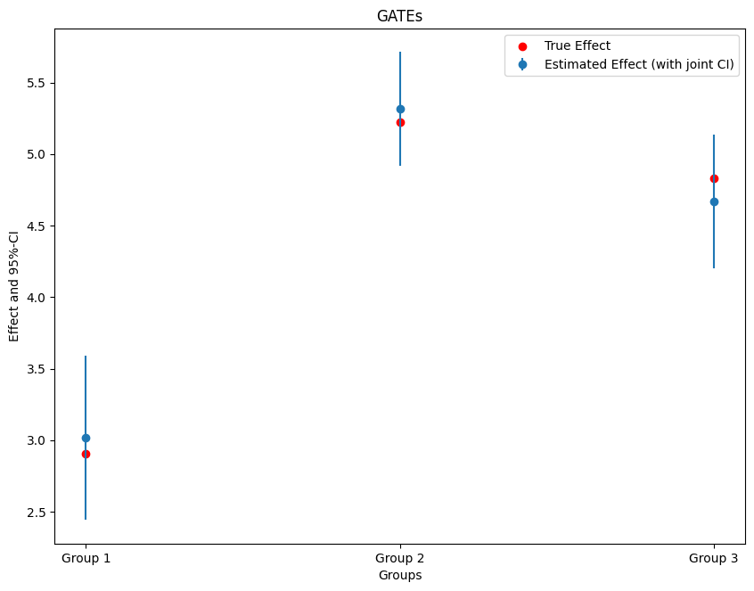
The confidence intervals above are point-wise, but by setting the option joint and providing a number of bootstrap repetitions n_rep_boot.

ci = gate.confint(level=0.95, joint=True, n_rep_boot=1000)
print(ci)

            2.5 %    effect    97.5 %
Group 1  2.441219  3.016315  3.591411
Group 2  4.916528  5.314651  5.712774
Group 3  4.199893  4.668981  5.138068

Finally, let us plot the estimates together with the true effect within each group.

import matplotlib.pyplot as plt
plt.rcParams['figure.figsize'] = 10., 7.5

errors = np.full((2, ci.shape[0]), np.nan)
errors[0, :] = ci['effect'] - ci['2.5 %']
errors[1, :] = ci['97.5 %'] - ci['effect']

plt.errorbar(ci.index, ci.effect, fmt='o', yerr=errors, label='Estimated Effect (with joint CI)')

#add true effect
ax = plt.subplot(1, 1, 1)
ax.scatter(x=['Group 1', 'Group 2', 'Group 3'], y=true_effects, c='red', label='True Effect')

plt.title('GATEs')
plt.xlabel('Groups')
plt.legend()
_ = plt.ylabel('Effect and 95%-CI')

It is also possible to supply disjoint groups as a single vector (still as a data frame). Remark the slightly different name.

groups =  pd.DataFrame(columns=['Group'], index=range(data['X_0'].shape[0]), dtype=str)
for i, x_i in enumerate(data['X_0']):
    if x_i <= 0.3:
         groups['Group'][i] = '1'
    elif (x_i > 0.3) & (x_i <= 0.7):
         groups['Group'][i] = '2'
    else:
         groups['Group'][i] = '3'

print(groups.head())

  Group
0     3
1     2
2     2
3     2
4     2

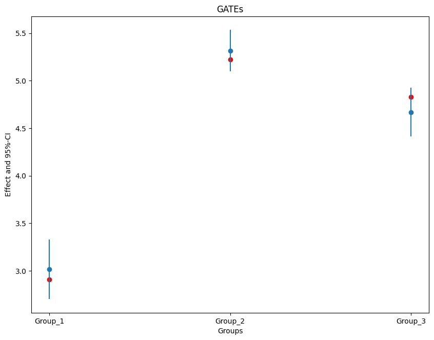
This time lets consider pointwise confidence intervals.

gate = dml_irm.gate(groups=groups)
ci = gate.confint()
print(ci)

            2.5 %    effect    97.5 %
Group_1  2.701265  3.016315  3.331365
Group_2  5.096550  5.314651  5.532751
Group_3  4.412004  4.668981  4.925957

The coefficients of the best linear predictor can be seen via the summary (the values can be accessed through the underlying model .blp_model).

print(gate.summary)

             coef   std err          t          P>|t|    [0.025    0.975]
Group_1  3.016315  0.144241  20.911662   3.948154e-70  2.732918  3.299712
Group_2  5.314651  0.117072  45.396300  6.151047e-179  5.084633  5.544669
Group_3  4.668981  0.138851  33.625766  3.991444e-130  4.396173  4.941788

Remark that the confidence intervals in the summary are slightly smaller, since they are not based on the White’s heteroskedasticity robus standard errors.

errors = np.full((2, ci.shape[0]), np.nan)
errors[0, :] = ci['effect'] - ci['2.5 %']
errors[1, :] = ci['97.5 %'] - ci['effect']

#add true effect
ax = plt.subplot(1, 1, 1)
ax.scatter(x=['Group_1', 'Group_2', 'Group_3'], y=true_effects, c='red', label='True Effect')

plt.errorbar(ci.index, ci.effect, fmt='o', yerr=errors)
plt.title('GATEs')
plt.xlabel('Groups')
_ =  plt.ylabel('Effect and 95%-CI')