Note

https://docs.doubleml.org/stable/examples/py_double_ml_policy_tree.ipynb

Python: Policy Learning with Trees#

In this simple example, we illustrate how the DoubleML package can be used to estimate deterministic binary treatment policies.

Data#

The data will be generated with a simple data generating process to enable us to know the true policy cut-offs.

[1]:

import numpy as np
import pandas as pd
import doubleml as dml

Here, we consider a treatment effect that depends on two covariates which might correspond to opposite effects depending on age or income. For simplicity, the treatment effect within each group is generated to be constant.

[2]:

def group_effect(x):
    if x[0] <= -0.3:
        te = 2.2
    elif (x[0] >= 0.2) & (x[1] >= 0.4):
        te = 2
    else:
        te = -2
    return te

The data is generated as

\[\begin{split}\begin{aligned} Y_i & = g(W_1,W_2)T_i + \langle W_i,\gamma_0\rangle + \epsilon_i \\ T_i & = \langle W_i,\beta_0\rangle +\eta_i, \end{aligned}\end{split}\]

where \(W_i\sim\mathcal{N}(0,I_{d_w})\) and \(\epsilon_i,\eta_i\sim\mathcal{U}[0,1]\). The coefficient vectors \(\gamma_0\) and \(\beta_0\) both have small random support which values are drawn independently from \(\mathcal{U}[0,1]\). Further, \(g(w_1,w_2)\) defines the conditional treatment effect, which is generated depending on \(\{w_1,w_2\}\).

\[\begin{split}g(w_1) = \begin{cases}2.2\quad &\text{for } w_1\le -0.3\\ 2\quad &\text{for } w_1\ge 0.2 \land w_2\ge 0.4\\ -2\quad &\text{otherwise. } \\ \end{cases}\end{split}\]

[3]:

def create_synthetic_group_data(n_samples=200, n_w=10, support_size=5):
    """
    Creates a simple synthetic example for group effects.

    Parameters
    ----------
    n_samples : int
        Number of samples.
        Default is ``200``.

    n_w : int
        Dimension of covariates.
        Default is ``10``.

    support_size : int
        Number of relevant covariates.
        Default is ``5``.

    Returns
    -------
     data : pd.DataFrame
            A data frame.

    """
    # Outcome support
    support_w = np.random.choice(np.arange(n_w), size=support_size, replace=False)
    coefs_w = np.random.uniform(0, 1, size=support_size)
    # Define the function to generate the noise
    epsilon_sample = lambda n: np.random.uniform(-1, 1, size=n_samples)
    # Treatment support
    # Assuming the matrices gamma and beta have the same number of non-zero components
    support_t = np.random.choice(np.arange(n_w), size=support_size, replace=False)
    coefs_t = np.random.uniform(0, 1, size=support_size)
    # Define the function to generate the noise
    eta_sample = lambda n: np.random.uniform(-1, 1, size=n_samples)

    # Generate controls, covariates, treatments and outcomes
    w = np.random.normal(0, 1, size=(n_samples, n_w))
    # Group treatment effect
    te = np.apply_along_axis(group_effect, axis=1, arr=w)
    # Define treatment
    log_odds = np.dot(w[:, support_t], coefs_t) + eta_sample(n_samples)
    t_sigmoid = 1 / (1 + np.exp(-log_odds))
    t = np.array([np.random.binomial(1, p) for p in t_sigmoid])
    # Define the outcome
    y = te * t + np.dot(w[:, support_w], coefs_w) + epsilon_sample(n_samples)

    # Now we build the dataset
    y_df = pd.DataFrame({'y': y})
    t_df = pd.DataFrame({'t': t})
    w_df = pd.DataFrame(data=w, index=np.arange(w.shape[0]),
                        columns=[f'w_{i}' for i in range(1, w.shape[1] + 1)])

    data = pd.concat([y_df, t_df, w_df], axis=1)
    covariates = list(w_df.columns.values)

    return data, covariates

We will consider a quite small number of covariates to ensure fast calcualtion.

[4]:

# DGP constants
np.random.seed(42)
n_samples = 500
n_w = 10
support_size = 5

# Create data
data, covariates = create_synthetic_group_data(n_samples=n_samples, n_w=n_w, support_size=support_size)
data_dml_base = dml.DoubleMLData(data,
                                 y_col='y',
                                 d_cols='t',
                                 x_cols=covariates)

Interactive Regression Model (IRM)#

The first step is to fit a DoubleML IRM Model to the data.

[5]:

# First stage estimation
from sklearn.ensemble import RandomForestClassifier, RandomForestRegressor
randomForest_reg = RandomForestRegressor(n_estimators=200, random_state=42)
randomForest_class = RandomForestClassifier(n_estimators=200, random_state=42)

np.random.seed(42)

dml_irm = dml.DoubleMLIRM(data_dml_base,
                          ml_g=randomForest_reg,
                          ml_m=randomForest_class,
                          trimming_threshold=0.01,
                          n_folds=5)
print("Training IRM Model")
dml_irm.fit(store_predictions=True)

Training IRM Model

[5]:

<doubleml.double_ml_irm.DoubleMLIRM at 0x2920d7b7150>

Policy Learning with Trees#

Next, we specify the covariates as a DataFrame against which to learn the policy. This can either be all covariates \(w_i\), or if domain knowledge is available we can use a subset.

[6]:

features = data[["w_1","w_2"]].copy()
print(features)

          w_1       w_2
0   -0.428046 -0.742407
1   -0.600254  0.947440
2   -1.265119  1.091992
3   -1.346678 -0.880591
4   -1.508153  1.099647
..        ...       ...
495 -2.072293 -0.951920
496  0.144908  0.280963
497 -0.877455 -2.404550
498 -0.981104 -0.830301
499 -0.555445  0.021866

[500 rows x 2 columns]

To estimate a Policy just call the policy_tree() method and supply the DataFrame with the features and the depth of the desired tree.

[7]:

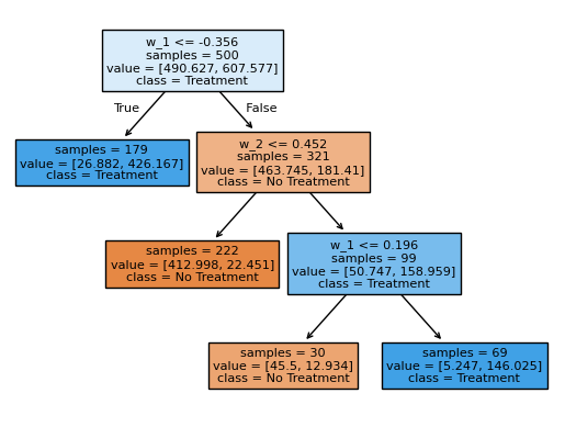
policy_tree = dml_irm.policy_tree(features=features, depth=3)
policy_tree.plot_tree();

../_images/examples_py_double_ml_policy_tree_14_0.png

The splits in this classification tree reflect the heterogeneity in the data generating process above. Exemplatory, we see that the first split is estimated at \(w_1 = -0.292\). In the DGP, at \(w_1 = -0.3\) the treatment effect jumps from \(-2\) to \(2.2\).

Alternatively, it is also possible to estimate the tree on all covariates, which in this case results in the same splits.

[8]:

policy_tree_2 = dml_irm.policy_tree(features=data[covariates], depth=3)
policy_tree_2.plot_tree();

../_images/examples_py_double_ml_policy_tree_17_0.png

The policytree predict() method is useful to estimate the optimal treatments on new data.

[9]:

new_data, _ = create_synthetic_group_data(n_samples=n_samples, n_w=n_w, support_size=support_size)
pred_df = policy_tree.predict(features=new_data[["w_1","w_2"]])
print(pred_df)

          w_1       w_2  pred_treatment
0   -1.155516  1.570111               1
1   -2.216761  1.389566               1
2    0.764478 -1.111164               0
3   -0.411291  0.984024               1
4    0.324518  1.675293               1
..        ...       ...             ...
495 -1.728294 -0.018023               1
496  0.632958  2.557731               1
497 -0.161198  0.661369               0
498  0.351766  0.523807               1
499 -0.366529  1.310761               1

[500 rows x 3 columns]

These predicted optimal treatments maximize the overall Average Treament Effect on the treated within the new data. We showcase that with the help of the gate() method.

[10]:

data_dml_new = dml.DoubleMLData(new_data,
                                y_col="y",
                                d_cols="t")

dml_irm_new = dml.DoubleMLIRM(data_dml_new,
                              ml_g=randomForest_reg,
                              ml_m=randomForest_class,
                              trimming_threshold=0.01,
                              n_folds=5)
dml_irm_new.fit()
print("ATTE under the original treatment policy:")
print(dml_irm_new.gate(groups=new_data["t"].to_frame()).confint())
print("\nATTE under the estimated optimal treatment policy:")
print(dml_irm_new.gate(groups=pred_df["pred_treatment"].to_frame()).confint())

ATTE under the original treatment policy:
      2.5 %    effect    97.5 %
t -0.192505  0.177463  0.547431

ATTE under the estimated optimal treatment policy:
                   2.5 %    effect    97.5 %
pred_treatment  1.712157  1.982797  2.253437

Using the original policy in the underlying DGP, we achieve a significant ATTE improvement.