Note
-
Download Jupyter notebook:
https://docs.doubleml.org/stable/examples/py_double_ml_cvar.ipynb.
Python: Conditional Value at Risk of potential outcomes#
In this example, we illustrate how the DoubleML package can be used to estimate the conditional Value at Risk of potential outcomes. The estimation is based on Kallus et al. (2019).
Data#
We define a data generating process to create synthetic data to compare the estimates to the true effect.
[1]:
import numpy as np
import pandas as pd
import doubleml as dml
import multiprocessing

from lightgbm import LGBMClassifier, LGBMRegressor
The data is generated as a location-scale model with
where \(X_i\sim\mathcal{U}[-1,1]^{p}\) and \(\varepsilon_i \sim \mathcal{N}(0,1)\). Further, the location and scale are determined according to the following functions
and the treatment takes the following form
with \(\epsilon_i \sim \mathcal{N}(0,1)\).
[2]:
def f_loc(D, X):
  loc = 0.5*D + 2*D*X[:,4] + 2.0*(X[:,1] > 0.1) - 1.7*(X[:,0] * X[:,2] > 0) - 3*X[:,3]
  return loc

def f_scale(D, X):
  scale = np.sqrt(0.5*D + 0.3*D*X[:,1] + 2)
  return scale

def dgp(n=200, p=5):
    X = np.random.uniform(-1,1,size=[n,p])
    D = ((X[:,1 ] - X[:,3] + 1.5*(X[:,0] > 0) + np.random.normal(size=n)) > 0)*1.0
    epsilon = np.random.normal(size=n)

    Y = f_loc(D, X) + f_scale(D, X)*epsilon

    return Y, X, D, epsilon
We can calculate the true conditional value at risk through simulations. Here, we will just approximate the true conditional value at risk for the potential outcomes for a range of quantiles.
[3]:
tau_vec = np.arange(0.1,0.95,0.05)
p = 5
n_true = int(10e+6)

_, X_true, _, epsilon_true = dgp(n=n_true, p = p)
D1 = np.ones(n_true)
D0 = np.zeros(n_true)

Y1 = f_loc(D1, X_true) + f_scale(D1, X_true)*epsilon_true
Y0 = f_loc(D0, X_true) + f_scale(D0, X_true)*epsilon_true

Y1_quant = np.quantile(Y1, q=tau_vec)
Y0_quant = np.quantile(Y0, q=tau_vec)

Y1_cvar = [Y1[Y1 >= quant].mean() for quant in Y1_quant]
Y0_cvar = [Y0[Y0 >= quant].mean() for quant in Y0_quant]

print(f'Conditional Value at Risk Y(0): {Y0_cvar}')
print(f'Conditional Value at Risk Y(1): {Y1_cvar}')
Conditional Value at Risk Y(0): [np.float64(0.5473064979425033), np.float64(0.756585519864526), np.float64(0.9574793755564219), np.float64(1.1539831483813536), np.float64(1.3486970271639334), np.float64(1.5436876323961168), np.float64(1.7407627053044026), np.float64(1.9417090334740552), np.float64(2.1484554868601506), np.float64(2.3631031251500065), np.float64(2.5883964619856044), np.float64(2.827874854703913), np.float64(3.086401570476133), np.float64(3.3711317415516624), np.float64(3.6934117220290754), np.float64(4.0735183279373635), np.float64(4.554986206618521)]
Conditional Value at Risk Y(1): [np.float64(1.1121351274811793), np.float64(1.3466832975109777), np.float64(1.5714294154804167), np.float64(1.7910908091075142), np.float64(2.008825189994473), np.float64(2.227018245501943), np.float64(2.447863428811719), np.float64(2.6734628878523097), np.float64(2.906051023766621), np.float64(3.1482102407485826), np.float64(3.403113188429014), np.float64(3.675011328023803), np.float64(3.969702563412915), np.float64(4.295855642811191), np.float64(4.667285944503316), np.float64(5.108783087402629), np.float64(5.673581815999206)]
Let us generate \(n=5000\) observations and convert them to a DoubleMLData object.
[4]:
n = 5000
np.random.seed(42)
Y, X, D, _ = dgp(n=n,p=p)
obj_dml_data = dml.DoubleMLData.from_arrays(X, Y, D)
Conditional Value at Risk (CVaR)#
Next, we can initialize our two machine learning algorithms to train the different nuisance elements (remark that in contrast to potential quantile estimation ml_g is a regressor). Then we can initialize the DoubleMLCVAR objects and call fit() to estimate the relevant parameters. To obtain confidence intervals, we can use the confint() method.
[5]:
ml_g = LGBMRegressor(n_estimators=300, learning_rate=0.05, num_leaves=10, verbose=-1, n_jobs=1)
ml_m = LGBMClassifier(n_estimators=300, learning_rate=0.05, num_leaves=10, verbose=-1, n_jobs=1)

CVAR_0 = np.full((len(tau_vec)), np.nan)
CVAR_1 = np.full((len(tau_vec)), np.nan)

ci_CVAR_0 = np.full((len(tau_vec),2), np.nan)
ci_CVAR_1 = np.full((len(tau_vec),2), np.nan)

for idx_tau, tau in enumerate(tau_vec):
    print(f'Quantile: {tau}')
    dml_CVAR_0 = dml.DoubleMLCVAR(obj_dml_data,
                                ml_g, ml_m,
                                quantile=tau,
                                treatment=0,
                                n_folds=5)
    dml_CVAR_1 = dml.DoubleMLCVAR(obj_dml_data,
                                ml_g, ml_m,
                                quantile=tau,
                                treatment=1,
                                n_folds=5)

    dml_CVAR_0.fit()
    dml_CVAR_1.fit()

    ci_CVAR_0[idx_tau, :] = dml_CVAR_0.confint(level=0.95).to_numpy()
    ci_CVAR_1[idx_tau, :] = dml_CVAR_1.confint(level=0.95).to_numpy()

    CVAR_0[idx_tau] = dml_CVAR_0.coef.squeeze()
    CVAR_1[idx_tau] = dml_CVAR_1.coef.squeeze()
Quantile: 0.1
Quantile: 0.15000000000000002
Quantile: 0.20000000000000004
Quantile: 0.25000000000000006
Quantile: 0.30000000000000004
Quantile: 0.3500000000000001
Quantile: 0.40000000000000013
Quantile: 0.45000000000000007
Quantile: 0.5000000000000001
Quantile: 0.5500000000000002
Quantile: 0.6000000000000002
Quantile: 0.6500000000000001
Quantile: 0.7000000000000002
Quantile: 0.7500000000000002
Quantile: 0.8000000000000002
Quantile: 0.8500000000000002
Quantile: 0.9000000000000002
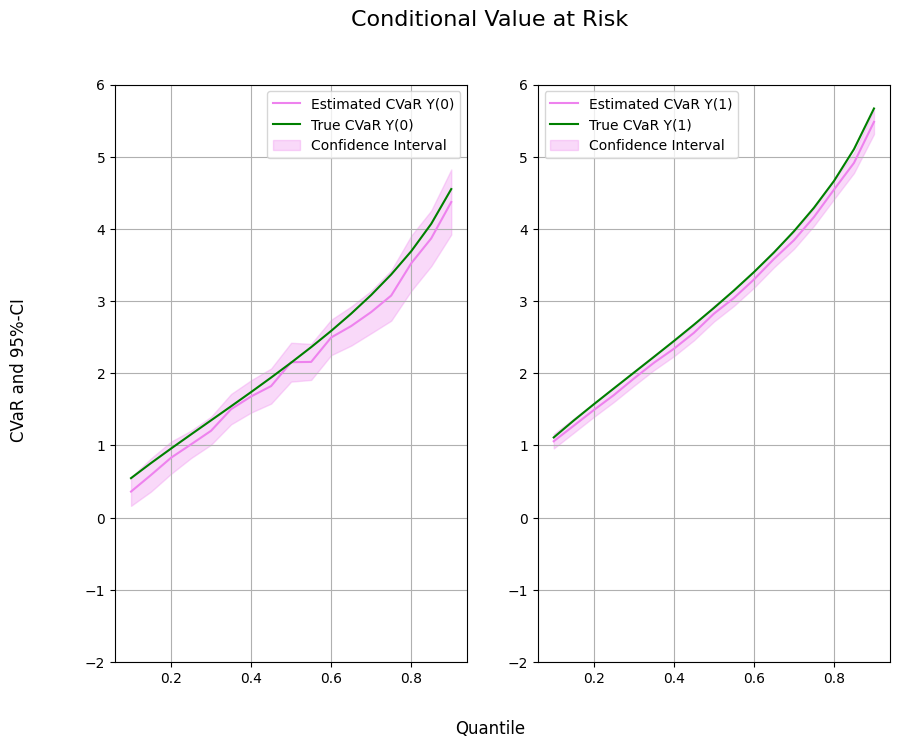
Finally, let us take a look at the estimated values.
[6]:
data = {"Quantile": tau_vec, "CVaR Y(0)": Y0_cvar, "CVaR Y(1)": Y1_cvar,
        "DML CVaR Y(0)": CVAR_0, "DML CVaR Y(1)": CVAR_1,
        "DML CVaR Y(0) lower": ci_CVAR_0[:, 0], "DML CVaR Y(0) upper": ci_CVAR_0[:, 1],
        "DML CVaR Y(1) lower": ci_CVAR_1[:, 0], "DML CVaR Y(1) upper": ci_CVAR_1[:, 1]}
df = pd.DataFrame(data)
print(df)
    Quantile  CVaR Y(0)  CVaR Y(1)  DML CVaR Y(0)  DML CVaR Y(1)  \
0       0.10   0.547306   1.112135       0.360683       1.057962
1       0.15   0.756586   1.346683       0.590911       1.273356
2       0.20   0.957479   1.571429       0.829543       1.489699
3       0.25   1.153983   1.791091       1.015038       1.697000
4       0.30   1.348697   2.008825       1.203284       1.925736
5       0.35   1.543688   2.227018       1.502494       2.144084
6       0.40   1.740763   2.447863       1.678826       2.338775
7       0.45   1.941709   2.673463       1.822482       2.559144
8       0.50   2.148455   2.906051       2.153119       2.824701
9       0.55   2.363103   3.148210       2.156969       3.041831
10      0.60   2.588396   3.403113       2.495657       3.298120
11      0.65   2.827875   3.675011       2.653846       3.582761
12      0.70   3.086402   3.969703       2.847948       3.842405
13      0.75   3.371132   4.295856       3.076347       4.163895
14      0.80   3.693412   4.667286       3.523163       4.543075
15      0.85   4.073518   5.108783       3.869020       4.913774
16      0.90   4.554986   5.673582       4.372097       5.482038

    DML CVaR Y(0) lower  DML CVaR Y(0) upper  DML CVaR Y(1) lower  \
0              0.162710             0.558655             0.957745
1              0.360801             0.821021             1.175284
2              0.606342             1.052745             1.393604
3              0.824889             1.205187             1.601061
4              1.009428             1.397140             1.824750
5              1.292028             1.712960             2.041147
6              1.455078             1.902573             2.234534
7              1.579238             2.065725             2.455107
8              1.883914             2.422325             2.715407
9              1.907491             2.406446             2.932027
10             2.250210             2.741104             3.183526
11             2.382872             2.924821             3.466440
12             2.554076             3.141820             3.722848
13             2.727976             3.424717             4.041284
14             3.140833             3.905494             4.409746
15             3.483717             4.254324             4.773177
16             3.921372             4.822822             5.313209

    DML CVaR Y(1) upper
0              1.158178
1              1.371429
2              1.585793
3              1.792939
4              2.026723
5              2.247020
6              2.443016
7              2.663182
8              2.933996
9              3.151636
10             3.412714
11             3.699082
12             3.961962
13             4.286507
14             4.676405
15             5.054370
16             5.650867
[7]:
from matplotlib import pyplot as plt
plt.rcParams['figure.figsize'] = 10., 7.5
fig, (ax1, ax2) = plt.subplots(1 ,2)
ax1.grid(); ax2.grid()

ax1.plot(df['Quantile'],df['DML CVaR Y(0)'], color='violet', label='Estimated CVaR Y(0)')
ax1.plot(df['Quantile'],df['CVaR Y(0)'], color='green', label='True CVaR Y(0)')
ax1.fill_between(df['Quantile'], df['DML CVaR Y(0) lower'], df['DML CVaR Y(0) upper'], color='violet', alpha=.3, label='Confidence Interval')
ax1.legend()
ax1.set_ylim(-2, 6)

ax2.plot(df['Quantile'],df['DML CVaR Y(1)'], color='violet', label='Estimated CVaR Y(1)')
ax2.plot(df['Quantile'],df['CVaR Y(1)'], color='green', label='True CVaR Y(1)')
ax2.fill_between(df['Quantile'], df['DML CVaR Y(1) lower'], df['DML CVaR Y(1) upper'], color='violet', alpha=.3, label='Confidence Interval')
ax2.legend()
ax2.set_ylim(-2, 6)

fig.suptitle('Conditional Value at Risk', fontsize=16)
fig.supxlabel('Quantile')
_ = fig.supylabel('CVaR and 95%-CI')
CVaR Treatment Effects#
In most cases, we want to evaluate the treatment effect on the CVaR as the difference between potential CVaRs. To estimate the treatment effect, we can use the DoubleMLQTE object and specify CVaR as the score.
As for quantile treatment effects, different quantiles can be estimated in parallel with n_jobs_models.
[8]:
n_cores = multiprocessing.cpu_count()
cores_used = np.min([5, n_cores - 1])
print(f"Number of Cores used: {cores_used}")

dml_CVAR = dml.DoubleMLQTE(obj_dml_data,
                           ml_g,
                           ml_m,
                           score='CVaR',
                           quantiles=tau_vec,
                           n_folds=5)
dml_CVAR.fit(n_jobs_models=cores_used)
print(dml_CVAR)
Number of Cores used: 5
================== DoubleMLQTE Object ==================

------------------ Fit summary       ------------------
          coef   std err         t         P>|t|     2.5 %    97.5 %
0.10  0.627564  0.103806  6.045553  1.488982e-09  0.424108  0.831019
0.15  0.677980  0.102616  6.606954  3.923084e-11  0.476856  0.879103
0.20  0.706645  0.100356  7.041387  1.903366e-12  0.509951  0.903339
0.25  0.716793  0.102775  6.974414  3.071543e-12  0.515358  0.918227
0.30  0.716762  0.107073  6.694154  2.169220e-11  0.506903  0.926621
0.35  0.740869  0.112216  6.602168  4.051870e-11  0.520930  0.960808
0.40  0.756969  0.114647  6.602628  4.039302e-11  0.532266  0.981672
0.45  0.751710  0.117710  6.386102  1.701672e-10  0.521002  0.982417
0.50  0.779682  0.122408  6.369556  1.895768e-10  0.539767  1.019596
0.55  0.786744  0.130370  6.034690  1.592681e-09  0.531223  1.042265
0.60  0.814351  0.138378  5.884996  3.980643e-09  0.543136  1.085566
0.65  0.848868  0.144800  5.862359  4.563374e-09  0.565066  1.132671
0.70  0.946968  0.154828  6.116274  9.578847e-10  0.643512  1.250425
0.75  0.997621  0.164805  6.053331  1.418806e-09  0.674609  1.320633
0.80  1.073520  0.190915  5.623024  1.876431e-08  0.699333  1.447706
0.85  1.053558  0.236008  4.464076  8.041491e-06  0.590991  1.516125
0.90  1.097468  0.338908  3.238251  1.202650e-03  0.433221  1.761714
As for standard DoubleMLCVAR objects, we can construct valid confidencebands with the confint() method. Additionally, it might be helpful to construct uniformly valid confidence regions via boostrap.
[9]:
ci_CVAR = dml_CVAR.confint(level=0.95, joint=False)

dml_CVAR.bootstrap(n_rep_boot=2000)
ci_joint_CVAR = dml_CVAR.confint(level=0.95, joint=True)
print(ci_joint_CVAR)
         2.5 %    97.5 %
0.10  0.367571  0.887556
0.15  0.420967  0.934992
0.20  0.455293  0.957996
0.25  0.459383  0.974202
0.30  0.448587  0.984937
0.35  0.459812  1.021926
0.40  0.469825  1.044113
0.45  0.456892  1.046527
0.50  0.473099  1.086264
0.55  0.460218  1.113270
0.60  0.467770  1.160932
0.65  0.486202  1.211534
0.70  0.559186  1.334750
0.75  0.584849  1.410393
0.80  0.595353  1.551686
0.85  0.462451  1.644665
0.90  0.248638  1.946297
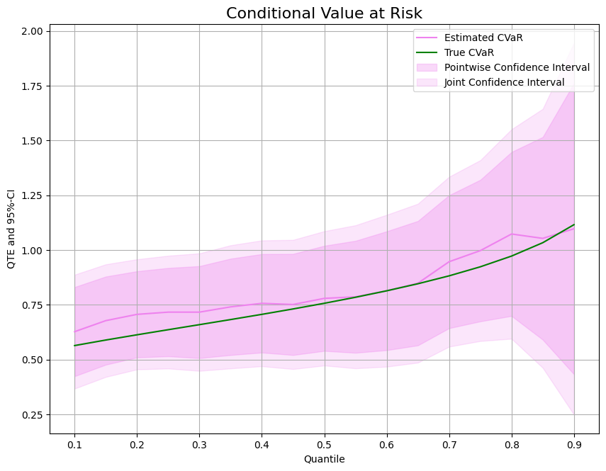
Finally, we can compare the predicted treatment effect with the true treatment effect on the CVaR.
[10]:
CVAR = np.array(Y1_cvar) - np.array(Y0_cvar)
data = {"Quantile": tau_vec, "CVaR": CVAR, "DML CVaR": dml_CVAR.coef,
        "DML CVaR pointwise lower": ci_CVAR['2.5 %'], "DML CVaR pointwise upper": ci_CVAR['97.5 %'],
        "DML CVaR joint lower": ci_joint_CVAR['2.5 %'], "DML CVaR joint upper": ci_joint_CVAR['97.5 %']}
df = pd.DataFrame(data)
print(df)
      Quantile      CVaR  DML CVaR  DML CVaR pointwise lower  \
0.10      0.10  0.564829  0.627564                  0.424108
0.15      0.15  0.590098  0.677980                  0.476856
0.20      0.20  0.613950  0.706645                  0.509951
0.25      0.25  0.637108  0.716793                  0.515358
0.30      0.30  0.660128  0.716762                  0.506903
0.35      0.35  0.683331  0.740869                  0.520930
0.40      0.40  0.707101  0.756969                  0.532266
0.45      0.45  0.731754  0.751710                  0.521002
0.50      0.50  0.757596  0.779682                  0.539767
0.55      0.55  0.785107  0.786744                  0.531223
0.60      0.60  0.814717  0.814351                  0.543136
0.65      0.65  0.847136  0.848868                  0.565066
0.70      0.70  0.883301  0.946968                  0.643512
0.75      0.75  0.924724  0.997621                  0.674609
0.80      0.80  0.973874  1.073520                  0.699333
0.85      0.85  1.035265  1.053558                  0.590991
0.90      0.90  1.118596  1.097468                  0.433221

      DML CVaR pointwise upper  DML CVaR joint lower  DML CVaR joint upper
0.10                  0.831019              0.367571              0.887556
0.15                  0.879103              0.420967              0.934992
0.20                  0.903339              0.455293              0.957996
0.25                  0.918227              0.459383              0.974202
0.30                  0.926621              0.448587              0.984937
0.35                  0.960808              0.459812              1.021926
0.40                  0.981672              0.469825              1.044113
0.45                  0.982417              0.456892              1.046527
0.50                  1.019596              0.473099              1.086264
0.55                  1.042265              0.460218              1.113270
0.60                  1.085566              0.467770              1.160932
0.65                  1.132671              0.486202              1.211534
0.70                  1.250425              0.559186              1.334750
0.75                  1.320633              0.584849              1.410393
0.80                  1.447706              0.595353              1.551686
0.85                  1.516125              0.462451              1.644665
0.90                  1.761714              0.248638              1.946297
[11]:
plt.rcParams['figure.figsize'] = 10., 7.5
fig, ax = plt.subplots()
ax.grid()

ax.plot(df['Quantile'],df['DML CVaR'], color='violet', label='Estimated CVaR')
ax.plot(df['Quantile'],df['CVaR'], color='green', label='True CVaR')
ax.fill_between(df['Quantile'], df['DML CVaR pointwise lower'], df['DML CVaR pointwise upper'], color='violet', alpha=.3, label='Pointwise Confidence Interval')
ax.fill_between(df['Quantile'], df['DML CVaR joint lower'], df['DML CVaR joint upper'], color='violet', alpha=.2, label='Joint Confidence Interval')

plt.legend()
plt.title('Conditional Value at Risk', fontsize=16)
plt.xlabel('Quantile')
_ = plt.ylabel('QTE and 95%-CI')