Note

Download Jupyter notebook: https://docs.doubleml.org/stable/examples/py_double_ml_ssm.ipynb.

Python: Sample Selection Models

In this example, we illustrate how the DoubleML package can be used to estimate the average treatment effect (ATE) under sample selection or outcome attrition. The estimation is based on a simulated DGP from Appendix E of Bia, Huber and Lafférs (2023).

Consider the following DGP:

\[\begin{split}\begin{align*} Y_i &= \theta_0 D_i + X_i'\beta_0 + \varepsilon_i,\\ S_i &= \mathbb{1}\{D_i + \gamma_0 Z_i + X_i'\beta_0 + \upsilon_i > 0\}, \\ D_i &= \mathbb{1}\{X_i'\beta_0 + \xi_i > 0\} \end{align*}\end{split}\]

where \(Y_i\) is observed if \(S_i=1\) with

\[X_i \sim N(0, \sigma^2_X), \quad Z_i \sim N(0, 1), \quad (\varepsilon,_i \nu_i) \sim N(0, \sigma^2_{\varepsilon, \nu}), \quad \xi_i \sim N(0, 1).\]

Let \(D_i\in\{0,1\}\) denote the treatment status of unit \(i\) and let \(Y_{i}\) be the outcome of interest of unit \(i\). Using the potential outcome notation, we can write \(Y_{i}(d)\) for the potential outcome of unit \(i\) and treatment status \(d\). Further, let \(X_i\) denote a vector of pre-treatment covariates.

Outcome missing at random (MAR)

Now consider the first setting, in which the outcomes are missing at random (MAR), according to assumptions in Bia, Huber and Lafférs (2023). Let the covariance matrix \(\sigma^2_X\) be such that \(a_{ij} = 0.5^{|i - j|}\), \(\gamma_0 = 0\), \(\sigma^2_{\varepsilon, \upsilon} = \begin{pmatrix} 1 & 0 \\ 0 & 1 \end{pmatrix}\) and finally, let the vector of coefficients \(\beta_0\) resemble a quadratic decay of coefficients importance; \(\beta_{0,j} = 0.4/j^2\) for \(j = 1, \ldots, p\).

Data

We will use the implemented data generating process make_ssm_data to generate data according to the simulation in Appendix E of Bia, Huber and Lafférs (2023). The true ATE in this DGP is equal to \(\theta_0=1\) (it can be changed by setting the parameter theta).

The data generating process make_ssm_data by default settings already returns a DoubleMLData object (however, it can return a pandas DataFrame or a NumPy array if return_type is specified accordingly). In this first setting, we are estimating the ATE under missingness at random, so we set mar=True. The selection indicator S can be set via s_col.

import numpy as np
from doubleml.datasets import make_ssm_data
import doubleml as dml

np.random.seed(42)
n_obs = 2000
df = make_ssm_data(n_obs=n_obs, mar=True, return_type='DataFrame')

dml_data = dml.DoubleMLData(df, 'y', 'd', s_col='s')
print(dml_data)

================== DoubleMLData Object ==================

------------------ Data summary      ------------------
Outcome variable: y
Treatment variable(s): ['d']
Covariates: ['X1', 'X2', 'X3', 'X4', 'X5', 'X6', 'X7', 'X8', 'X9', 'X10', 'X11', 'X12', 'X13', 'X14', 'X15', 'X16', 'X17', 'X18', 'X19', 'X20', 'X21', 'X22', 'X23', 'X24', 'X25', 'X26', 'X27', 'X28', 'X29', 'X30', 'X31', 'X32', 'X33', 'X34', 'X35', 'X36', 'X37', 'X38', 'X39', 'X40', 'X41', 'X42', 'X43', 'X44', 'X45', 'X46', 'X47', 'X48', 'X49', 'X50', 'X51', 'X52', 'X53', 'X54', 'X55', 'X56', 'X57', 'X58', 'X59', 'X60', 'X61', 'X62', 'X63', 'X64', 'X65', 'X66', 'X67', 'X68', 'X69', 'X70', 'X71', 'X72', 'X73', 'X74', 'X75', 'X76', 'X77', 'X78', 'X79', 'X80', 'X81', 'X82', 'X83', 'X84', 'X85', 'X86', 'X87', 'X88', 'X89', 'X90', 'X91', 'X92', 'X93', 'X94', 'X95', 'X96', 'X97', 'X98', 'X99', 'X100']
Instrument variable(s): None
Selection variable: s
No. Observations: 2000

------------------ DataFrame info    ------------------
<class 'pandas.core.frame.DataFrame'>
RangeIndex: 2000 entries, 0 to 1999
Columns: 103 entries, X1 to s
dtypes: float64(103)
memory usage: 1.6 MB

Estimation

To estimate the ATE under sample selection, we will use the DoubleMLSSM class.

As for all DoubleML classes, we have to specify learners, which have to be initialized first. Given the simulated quadratic decay of coefficients importance, Lasso regression should be a suitable option (as for propensity scores, this will be a \(\mathcal{l}_1\)-penalized Logistic Regression).

The learner ml_g is used to fit conditional expectations of the outcome \(\mathbb{E}[Y_i|D_i, S_i, X_i]\), whereas the learners ml_m and ml_pi will be used to estimate the treatment and selection propensity scores \(P(D_i=1|X_i)\) and \(P(S_i=1|D_i, X_i)\).

from sklearn.linear_model import LassoCV, LogisticRegressionCV

ml_g = LassoCV()
ml_m = LogisticRegressionCV(penalty='l1', solver='liblinear')
ml_pi = LogisticRegressionCV(penalty='l1', solver='liblinear')

The DoubleMLSSM class can be used as any other DoubleML class.

The score is set to score='missing-at-random', since the parameters of the DGP were set to satisfy the assumptions of outcomes missing at random. Further, since the simulation in Bia, Huber and Lafférs (2023) uses normalization of inverse probability weights, we will apply the same setting by normalize_ipw=True.

After initialization, we have to call the fit() method to estimate the nuisance elements.

dml_ssm = dml.DoubleMLSSM(dml_data, ml_g, ml_m, ml_pi, score='missing-at-random', normalize_ipw=True)
dml_ssm.fit()

print(dml_ssm)

================== DoubleMLSSM Object ==================

------------------ Data summary      ------------------
Outcome variable: y
Treatment variable(s): ['d']
Covariates: ['X1', 'X2', 'X3', 'X4', 'X5', 'X6', 'X7', 'X8', 'X9', 'X10', 'X11', 'X12', 'X13', 'X14', 'X15', 'X16', 'X17', 'X18', 'X19', 'X20', 'X21', 'X22', 'X23', 'X24', 'X25', 'X26', 'X27', 'X28', 'X29', 'X30', 'X31', 'X32', 'X33', 'X34', 'X35', 'X36', 'X37', 'X38', 'X39', 'X40', 'X41', 'X42', 'X43', 'X44', 'X45', 'X46', 'X47', 'X48', 'X49', 'X50', 'X51', 'X52', 'X53', 'X54', 'X55', 'X56', 'X57', 'X58', 'X59', 'X60', 'X61', 'X62', 'X63', 'X64', 'X65', 'X66', 'X67', 'X68', 'X69', 'X70', 'X71', 'X72', 'X73', 'X74', 'X75', 'X76', 'X77', 'X78', 'X79', 'X80', 'X81', 'X82', 'X83', 'X84', 'X85', 'X86', 'X87', 'X88', 'X89', 'X90', 'X91', 'X92', 'X93', 'X94', 'X95', 'X96', 'X97', 'X98', 'X99', 'X100']
Instrument variable(s): None
Selection variable: s
No. Observations: 2000

------------------ Score & algorithm ------------------
Score function: missing-at-random

------------------ Machine learner   ------------------
Learner ml_g: LassoCV()
Learner ml_pi: LogisticRegressionCV(penalty='l1', solver='liblinear')
Learner ml_m: LogisticRegressionCV(penalty='l1', solver='liblinear')
Out-of-sample Performance:
Learner ml_g_d0 RMSE: [[1.10039862]]
Learner ml_g_d1 RMSE: [[1.11071087]]
Learner ml_pi RMSE: [[0.42388745]]
Learner ml_m RMSE: [[0.47222159]]

------------------ Resampling        ------------------
No. folds: 5
No. repeated sample splits: 1

------------------ Fit summary       ------------------
       coef  std err        t          P>|t|    2.5 %    97.5 %
d  0.997494  0.03113  32.0428  2.765710e-225  0.93648  1.058508

Confidence intervals at different levels can be obtained via

print(dml_ssm.confint(level=0.90))

     5.0 %    95.0 %
d  0.94629  1.048699

ATE estimates distribution

Here, we add a small simulation where we generate multiple datasets, estimate the ATE and collect the results (this may take some time).

n_rep = 200
ATE = 1.0

ATE_estimates = np.full((n_rep), np.nan)

np.random.seed(42)
for i_rep in range(n_rep):
    if (i_rep % int(n_rep/10)) == 0:
        print(f'Iteration: {i_rep}/{n_rep}')
    dml_data = make_ssm_data(n_obs=n_obs, mar=True)
    dml_ssm = dml.DoubleMLSSM(dml_data, ml_g, ml_m, ml_pi, score='missing-at-random', normalize_ipw=True)
    dml_ssm.fit()

    ATE_estimates[i_rep] = dml_ssm.coef.squeeze()

Iteration: 0/200
Iteration: 20/200
Iteration: 40/200
Iteration: 60/200
Iteration: 80/200
Iteration: 100/200
Iteration: 120/200
Iteration: 140/200
Iteration: 160/200
Iteration: 180/200

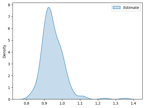
The distribution of the estimates takes the following form

import pandas as pd
import matplotlib.pyplot as plt
import seaborn as sns

df_pa = pd.DataFrame(ATE_estimates, columns=['Estimate'])
g = sns.kdeplot(df_pa, fill=True)
plt.show()

Outcome missing under nonignorable nonresponse

Now consider a different setting, in which the outcomes are missing under nonignorable nonresponse assumptions in Bia, Huber and Lafférs (2023). Let the covariance matrix \(\sigma^2_X\) again be such that \(a_{ij} = 0.5^{|i - j|}\), but now \(\gamma_0 = 1\) and \(\sigma^2_{\varepsilon, \upsilon} = \begin{pmatrix} 1 & 0.8 \\ 0.8 & 1 \end{pmatrix}\) to show a strong correlation between \(\varepsilon\) and \(\upsilon\). Let the vector of coefficients \(\beta\) again resemble a quadratic decay of coefficients importance; \(\beta_{0,j} = 0.4/j^2\) for \(j = 1, \ldots, p\).

The directed acyclic graph (DAG) shows the the structure of the causal model.

Data

We will again use the implemented data generating process make_ssm_data to generate data according to the simulation in Appendix E of Bia, Huber and Lafférs (2023). We will again leave the default ATE equal to \(\theta_0=1\).

In this setting, we are estimating the ATE under nonignorable nonresponse, so we set mar=False. Again, the selection indicator S can be set via s_col. Further, we need to specify an intrument via z_col.

np.random.seed(42)
n_obs = 8000
df = make_ssm_data(n_obs=n_obs, mar=False, return_type='DataFrame')
dml_data = dml.DoubleMLData(df, 'y', 'd', z_cols='z', s_col='s')
print(dml_data)

================== DoubleMLData Object ==================

------------------ Data summary      ------------------
Outcome variable: y
Treatment variable(s): ['d']
Covariates: ['X1', 'X2', 'X3', 'X4', 'X5', 'X6', 'X7', 'X8', 'X9', 'X10', 'X11', 'X12', 'X13', 'X14', 'X15', 'X16', 'X17', 'X18', 'X19', 'X20', 'X21', 'X22', 'X23', 'X24', 'X25', 'X26', 'X27', 'X28', 'X29', 'X30', 'X31', 'X32', 'X33', 'X34', 'X35', 'X36', 'X37', 'X38', 'X39', 'X40', 'X41', 'X42', 'X43', 'X44', 'X45', 'X46', 'X47', 'X48', 'X49', 'X50', 'X51', 'X52', 'X53', 'X54', 'X55', 'X56', 'X57', 'X58', 'X59', 'X60', 'X61', 'X62', 'X63', 'X64', 'X65', 'X66', 'X67', 'X68', 'X69', 'X70', 'X71', 'X72', 'X73', 'X74', 'X75', 'X76', 'X77', 'X78', 'X79', 'X80', 'X81', 'X82', 'X83', 'X84', 'X85', 'X86', 'X87', 'X88', 'X89', 'X90', 'X91', 'X92', 'X93', 'X94', 'X95', 'X96', 'X97', 'X98', 'X99', 'X100']
Instrument variable(s): ['z']
Selection variable: s
No. Observations: 8000

------------------ DataFrame info    ------------------
<class 'pandas.core.frame.DataFrame'>
RangeIndex: 8000 entries, 0 to 7999
Columns: 104 entries, X1 to s
dtypes: float64(104)
memory usage: 6.3 MB

Estimation

We will again use the DoubleMLSSM class.

Further, will leave he learners for all nuisance functions to be the same as in the first setting, as the simulated quadratic decay of coefficients importance still holds.

Now the learner ml_g is used to fit conditional expectations of the outcome \(\mathbb{E}[Y_i|D_i, S_i, X_i, \Pi_i]\), whereas the learners ml_m and ml_pi will be used to estimate the treatment and selection propensity scores \(P(D_i=1|X_i, \Pi_i)\) and \(P(S_i=1|D_i, X_i, Z_i)\).

ml_g = LassoCV()
ml_m = LogisticRegressionCV(penalty='l1', solver='liblinear')
ml_pi = LogisticRegressionCV(penalty='l1', solver='liblinear')

The score is now set to 'nonignorable', since the parameters of the DGP were set to satisfy the assumptions of outcomes missing under nonignorable nonresponse.

np.random.seed(42)
dml_ssm = dml.DoubleMLSSM(dml_data, ml_g, ml_m, ml_pi, score='nonignorable')
dml_ssm.fit()

print(dml_ssm)

================== DoubleMLSSM Object ==================

------------------ Data summary      ------------------
Outcome variable: y
Treatment variable(s): ['d']
Covariates: ['X1', 'X2', 'X3', 'X4', 'X5', 'X6', 'X7', 'X8', 'X9', 'X10', 'X11', 'X12', 'X13', 'X14', 'X15', 'X16', 'X17', 'X18', 'X19', 'X20', 'X21', 'X22', 'X23', 'X24', 'X25', 'X26', 'X27', 'X28', 'X29', 'X30', 'X31', 'X32', 'X33', 'X34', 'X35', 'X36', 'X37', 'X38', 'X39', 'X40', 'X41', 'X42', 'X43', 'X44', 'X45', 'X46', 'X47', 'X48', 'X49', 'X50', 'X51', 'X52', 'X53', 'X54', 'X55', 'X56', 'X57', 'X58', 'X59', 'X60', 'X61', 'X62', 'X63', 'X64', 'X65', 'X66', 'X67', 'X68', 'X69', 'X70', 'X71', 'X72', 'X73', 'X74', 'X75', 'X76', 'X77', 'X78', 'X79', 'X80', 'X81', 'X82', 'X83', 'X84', 'X85', 'X86', 'X87', 'X88', 'X89', 'X90', 'X91', 'X92', 'X93', 'X94', 'X95', 'X96', 'X97', 'X98', 'X99', 'X100']
Instrument variable(s): ['z']
Selection variable: s
No. Observations: 8000

------------------ Score & algorithm ------------------
Score function: nonignorable

------------------ Machine learner   ------------------
Learner ml_g: LassoCV()
Learner ml_pi: LogisticRegressionCV(penalty='l1', solver='liblinear')
Learner ml_m: LogisticRegressionCV(penalty='l1', solver='liblinear')
Out-of-sample Performance:
Learner ml_g_d0 RMSE: [[1.01990373]]
Learner ml_g_d1 RMSE: [[1.19983954]]
Learner ml_pi RMSE: [[0.37231324]]
Learner ml_m RMSE: [[0.43374433]]

------------------ Resampling        ------------------
No. folds: 5
No. repeated sample splits: 1

------------------ Fit summary       ------------------
       coef   std err          t          P>|t|  2.5 %    97.5 %
d  0.923517  0.037509  24.620995  7.528381e-134   0.85  0.997034

ATE estimates distribution

Here we again add a small simulation where we generate multiple datasets, estimate the ATE and collect the results (this may take some time).

ml_g = LassoCV()
ml_m = LogisticRegressionCV(penalty='l1', solver='liblinear')
ml_pi = LogisticRegressionCV(penalty='l1', solver='liblinear')


n_rep = 200
ATE = 1.0

ATE_estimates = np.full((n_rep), np.nan)

np.random.seed(42)
for i_rep in range(n_rep):
    if (i_rep % int(n_rep/10)) == 0:
        print(f'Iteration: {i_rep}/{n_rep}')
    dml_data = make_ssm_data(n_obs=n_obs, mar=False)
    dml_ssm = dml.DoubleMLSSM(dml_data, ml_g, ml_m, ml_pi, score='nonignorable')
    dml_ssm.fit()

    ATE_estimates[i_rep] = dml_ssm.coef.squeeze()

Iteration: 0/200
Iteration: 20/200
Iteration: 40/200
Iteration: 60/200
Iteration: 80/200
Iteration: 100/200
Iteration: 120/200
Iteration: 140/200
Iteration: 160/200
Iteration: 180/200

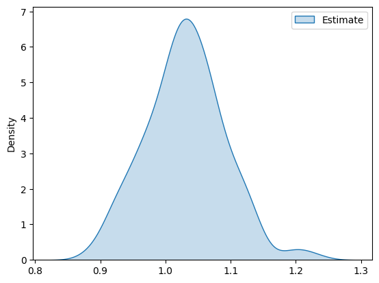
And plot the estimates distribution

df_pa = pd.DataFrame(ATE_estimates, columns=['Estimate'])
g = sns.kdeplot(df_pa, fill=True)
plt.show()