Note
-
Download Jupyter notebook:
https://docs.doubleml.org/stable/examples/learners/py_optuna.ipynb.
Python: Hyperparametertuning with Optuna#
This notebook explains how to use the implmented tune_ml_models() method to tune hyperparameters using the Optuna package.
In this example, we will focus on the DoubleMLAPO model to estimate average potential outcomes (APOs) in an interactive regression model (see DoubleMLIRM).
The goal is to estimate the average potential outcome
for a given treatment level \(d\) and and discrete valued treatment \(D\).
For a more detailed description of the DoubleMLAPO model, see Average Potential Outcome Model or Example Gallery.
Remark that the untuned settings and hyperparameter spaces are mainly chosen for display of the tuning possibilities and not a blueprint for standard tuning.
[1]:
import optuna
import numpy as np
import pandas as pd
import matplotlib.pyplot as plt
import seaborn as sns
from plotly.io import show

from sklearn.pipeline import Pipeline
from sklearn.preprocessing import RobustScaler
from sklearn.linear_model import LinearRegression, Ridge, LogisticRegression
from sklearn.ensemble import StackingRegressor, StackingClassifier
from lightgbm import LGBMRegressor, LGBMClassifier

from doubleml.data import DoubleMLData
from doubleml.irm import DoubleMLAPO, DoubleMLAPOS
from doubleml.irm.datasets import make_irm_data_discrete_treatments

palette = sns.color_palette("colorblind")

import warnings
warnings.filterwarnings("ignore")
Data Generating Process (DGP)#
At first, let us generate data according to the make_irm_data_discrete_treatments data generating process. The process generates data with a continuous treatment variable and contains the true individual treatment effects (ITEs) with respect to option of not getting treated.
According to the continuous treatment variable, the treatment is discretized into multiple levels, based on quantiles. Using the oracle ITEs, enables the comparison to the true APOs and averate treatment effects (ATEs) for the different levels of the treatment variable.
Remark: The average potential outcome model does not require an underlying continuous treatment variable. The model will work identically if the treatment variable is discrete by design.
[2]:
# Parameters
n_obs = 500
n_levels = 3
treatment_lvl = 1.0

np.random.seed(42)
data_apo = make_irm_data_discrete_treatments(n_obs=n_obs,n_levels=n_levels, linear=False)

y0 = data_apo['oracle_values']['y0']
cont_d = data_apo['oracle_values']['cont_d']
ite = data_apo['oracle_values']['ite']
d = data_apo['d']
potential_level = data_apo['oracle_values']['potential_level']
level_bounds = data_apo['oracle_values']['level_bounds']

average_ites = np.full(n_levels + 1, np.nan)
apos = np.full(n_levels + 1, np.nan)
mid_points = np.full(n_levels, np.nan)

for i in range(n_levels + 1):
    average_ites[i] = np.mean(ite[d == i]) * (i > 0)
    apos[i] = np.mean(y0) + average_ites[i]

print(f"Average Individual effects in each group:\n{np.round(average_ites,2)}\n")
print(f"Average Potential Outcomes in each group:\n{np.round(apos,2)}\n")
print(f"Levels and their counts:\n{np.unique(d, return_counts=True)}")
Average Individual effects in each group:
[ 0.    3.44  9.32 10.49]

Average Potential Outcomes in each group:
[210.05 213.49 219.38 220.54]

Levels and their counts:
(array([0., 1., 2., 3.]), array([171, 110, 109, 110]))
As for all DoubleML models, we specify a DoubleMLData object to handle the data.
[3]:
y = data_apo['y']
x = data_apo['x']
d = data_apo['d']
df_apo = pd.DataFrame(
    np.column_stack((y, d, x)),
    columns=['y', 'd'] + ['x' + str(i) for i in range(data_apo['x'].shape[1])]
)

dml_data = DoubleMLData(df_apo, 'y', 'd')
print(dml_data)
================== DoubleMLData Object ==================

------------------ Data summary      ------------------
Outcome variable: y
Treatment variable(s): ['d']
Covariates: ['x0', 'x1', 'x2', 'x3', 'x4']
Instrument variable(s): None
No. Observations: 500

------------------ DataFrame info    ------------------
<class 'pandas.core.frame.DataFrame'>
RangeIndex: 500 entries, 0 to 499
Columns: 7 entries, y to x4
dtypes: float64(7)
memory usage: 27.5 KB
Basic Tuning Example#
At first, we will take a look at a very basic tuning example without much customization.
Define Nuisance Learners#
For our example, we will choose LightGBM learners, which are typical non-parametric choice.
[4]:
ml_g = LGBMRegressor(random_state=314, verbose=-1)
ml_m = LGBMClassifier(random_state=314, verbose=-1)
Untuned Model#
Now let us take a look at the standard workflow, focusing on a single treatment level and using default hyperparameters.
[5]:
dml_obj_untuned = DoubleMLAPO(
    dml_data,
    ml_g,
    ml_m,
    treatment_level=treatment_lvl,
)

dml_obj_untuned.fit()
dml_obj_untuned.summary
[5]:
| coef | std err | t | P>|t| | 2.5 % | 97.5 % | |
|---|---|---|---|---|---|---|
| d | 211.232659 | 15.657431 | 13.490888 | 1.769555e-41 | 180.544657 | 241.920661 |
Hyperparameter Tuning#
Now, let us take a look at the basic hyperparameter tuning. We will initialize a separate model to compare the results.
[6]:
dml_obj_tuned = DoubleMLAPO(
    dml_data,
    ml_g,
    ml_m,
    treatment_level=treatment_lvl,
)
The required input for tuning is a parameter space dictionary for the hyperparameters for each learner that should be tuned. This dictionary should include a callable for each learner you want to have (only a subset is also possible, i.e. only tuning ml_g).
The parameter spaces should be a callable and suggest the search spaces via a trial object.
Generally, the hyperparameter structure should follow the definitions in Optuna, but instead of the objective the hyperparameters have to be specified as a callable. The corresponding DoubleML object then assigns a corresponding objective for each learning using the supplied parameter space.
To keep this example relatively fast and simple, we keep the n_estimators fix and only tune a small number of other hyperparameters.
[7]:
# parameter space for the outcome regression tuning
def ml_g_params(trial):
    return {
        'n_estimators': 100,
        'learning_rate': trial.suggest_float('learning_rate', 0.001, 0.1, log=True),
        'max_depth': 5,
        'min_child_samples': trial.suggest_int('min_child_samples', 20, 50, step=10),
        'lambda_l1': trial.suggest_float('lambda_l1', 1e-2, 10.0, log=True),
        'lambda_l2': trial.suggest_float('lambda_l2', 1e-2, 10.0, log=True),
    }

# parameter space for the propensity score tuning
def ml_m_params(trial):
    return {
        'n_estimators': 100,
        'learning_rate': trial.suggest_float('learning_rate', 0.001, 0.1, log=True),
        'max_depth': 5,
        'min_child_samples': trial.suggest_int('min_child_samples', 20, 50, step=10),
        'lambda_l1': trial.suggest_float('lambda_l1', 1e-2, 10.0, log=True),
        'lambda_l2': trial.suggest_float('lambda_l2', 1e-2, 10.0, log=True),
    }

param_space = {
    'ml_g': ml_g_params,
    'ml_m': ml_m_params
}
To tune the hyperparameters the tune_ml_models() with the ml_param_space argument should be called. Further, to define the number of trials and other optuna options you can use the optuna_setttings argument.
[8]:
optuna_settings = {
    'n_trials': 200,
    'show_progress_bar': True,
    'verbosity': optuna.logging.WARNING,  # Suppress Optuna logs
}

dml_obj_tuned.tune_ml_models(
    ml_param_space=param_space,
    optuna_settings=optuna_settings,
)
[8]:
<doubleml.irm.apo.DoubleMLAPO at 0x7f029668ba10>
Per default, the model will set the best hyperparameters automatically (identical hyperparameters for each fold), and you can directly call the fit() method afterwards.
[9]:
dml_obj_tuned.fit()
dml_obj_tuned.summary
[9]:
| coef | std err | t | P>|t| | 2.5 % | 97.5 % | |
|---|---|---|---|---|---|---|
| d | 215.273433 | 2.485 | 86.62916 | 0.0 | 210.402924 | 220.143943 |
Remark: Even if the initialization and tuning only requires the learners ml_g and ml_m, the models in the irm submodule generally, copy the learner for ml_g and fit different response surfaces for treatment and control (or not-treatment) groups. These different learners are tuned separately but with the same parameter space. To see which parameter spaces can be tuned you can take a look at the params_names property.
In this example, we specified the parameter spaces for ml_m and ml_g, but actually three sets of hyperparameters were tuned, i.e. ml_m, ml_g_d_lvl0 and ml_g_d_lvl1 (two response surfaces for the outcome).
[10]:
dml_obj_tuned.params_names
[10]:
['ml_g_d_lvl0', 'ml_g_d_lvl1', 'ml_m']
Each hyperparameter combination is set for each fold.
[11]:
dml_obj_tuned.params
[11]:
{'ml_g_d_lvl0': {'d': [[{'learning_rate': 0.09801463544687879,
     'min_child_samples': 20,
     'lambda_l1': 3.1247297280098136,
     'lambda_l2': 0.1676705013704926},
    {'learning_rate': 0.09801463544687879,
     'min_child_samples': 20,
     'lambda_l1': 3.1247297280098136,
     'lambda_l2': 0.1676705013704926},
    {'learning_rate': 0.09801463544687879,
     'min_child_samples': 20,
     'lambda_l1': 3.1247297280098136,
     'lambda_l2': 0.1676705013704926},
    {'learning_rate': 0.09801463544687879,
     'min_child_samples': 20,
     'lambda_l1': 3.1247297280098136,
     'lambda_l2': 0.1676705013704926},
    {'learning_rate': 0.09801463544687879,
     'min_child_samples': 20,
     'lambda_l1': 3.1247297280098136,
     'lambda_l2': 0.1676705013704926}]]},
 'ml_g_d_lvl1': {'d': [[{'learning_rate': 0.09957868943595276,
     'min_child_samples': 20,
     'lambda_l1': 1.0312190390696285,
     'lambda_l2': 0.058903541934281406},
    {'learning_rate': 0.09957868943595276,
     'min_child_samples': 20,
     'lambda_l1': 1.0312190390696285,
     'lambda_l2': 0.058903541934281406},
    {'learning_rate': 0.09957868943595276,
     'min_child_samples': 20,
     'lambda_l1': 1.0312190390696285,
     'lambda_l2': 0.058903541934281406},
    {'learning_rate': 0.09957868943595276,
     'min_child_samples': 20,
     'lambda_l1': 1.0312190390696285,
     'lambda_l2': 0.058903541934281406},
    {'learning_rate': 0.09957868943595276,
     'min_child_samples': 20,
     'lambda_l1': 1.0312190390696285,
     'lambda_l2': 0.058903541934281406}]]},
 'ml_m': {'d': [[{'learning_rate': 0.0732109605604835,
     'min_child_samples': 30,
     'lambda_l1': 9.590467244372398,
     'lambda_l2': 0.078138007883929},
    {'learning_rate': 0.0732109605604835,
     'min_child_samples': 30,
     'lambda_l1': 9.590467244372398,
     'lambda_l2': 0.078138007883929},
    {'learning_rate': 0.0732109605604835,
     'min_child_samples': 30,
     'lambda_l1': 9.590467244372398,
     'lambda_l2': 0.078138007883929},
    {'learning_rate': 0.0732109605604835,
     'min_child_samples': 30,
     'lambda_l1': 9.590467244372398,
     'lambda_l2': 0.078138007883929},
    {'learning_rate': 0.0732109605604835,
     'min_child_samples': 30,
     'lambda_l1': 9.590467244372398,
     'lambda_l2': 0.078138007883929}]]}}
Comparison#
Let us compare the results for both models. If we take a look at the predictive performance of the learners, the main difference can be observed in the log loss of the propensity score ml_m
[12]:
dml_obj_untuned.evaluate_learners()
[12]:
{'ml_g_d_lvl0': array([[14.49934441]]),
 'ml_g_d_lvl1': array([[23.50828321]]),
 'ml_m': array([[0.44349955]])}
[13]:
dml_obj_tuned.evaluate_learners()
[13]:
{'ml_g_d_lvl0': array([[14.73579164]]),
 'ml_g_d_lvl1': array([[23.25821083]]),
 'ml_m': array([[0.4101895]])}
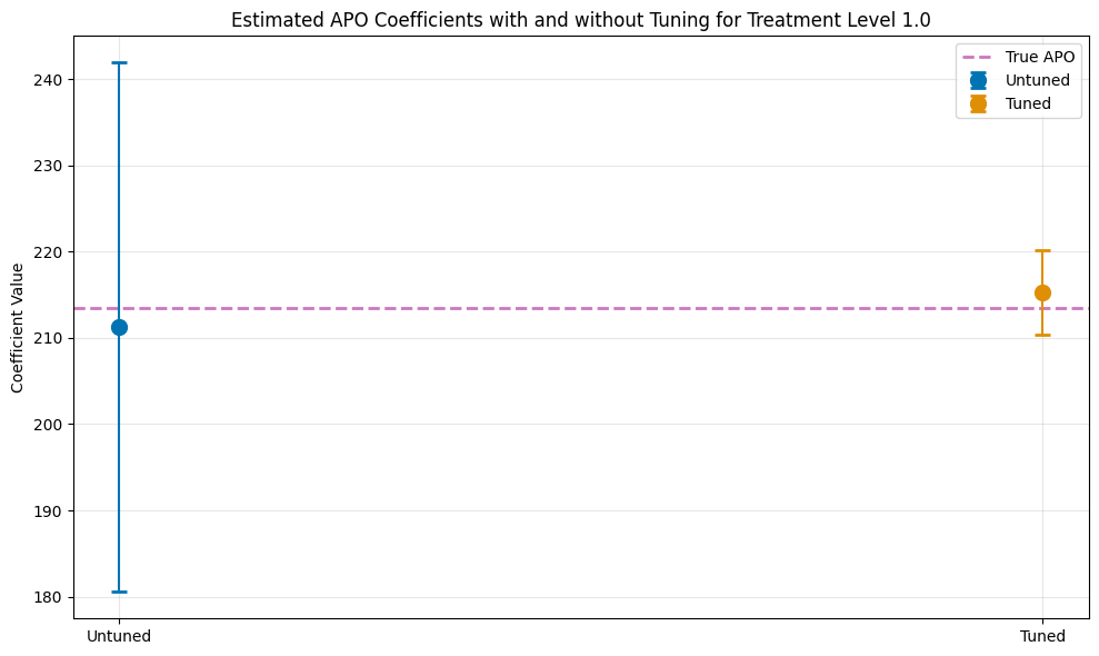
As a result the standard error is reduced and confidence intervals are much tighter.
[14]:
ci_untuned = dml_obj_untuned.confint()
ci_tuned = dml_obj_tuned.confint()

# Create comparison dataframe
comparison_data = {
    'Model': ['Untuned', 'Tuned'],
    'theta': [dml_obj_untuned.coef[0], dml_obj_tuned.coef[0]],
    'se': [dml_obj_untuned.se[0], dml_obj_tuned.se[0]],
    'ci_lower': [ci_untuned.iloc[0, 0], ci_tuned.iloc[0, 0]],
    'ci_upper': [ci_untuned.iloc[0, 1], ci_tuned.iloc[0, 1]]
}
df_comparison = pd.DataFrame(comparison_data)

print(f"\nTrue APO at treatment level {treatment_lvl}: {apos[int(treatment_lvl)]:.4f}\n")
print(df_comparison.to_string(index=False))

plt.figure(figsize=(10, 6))
plt.errorbar(0, df_comparison.loc[0, 'theta'],
             yerr=[[df_comparison.loc[0, 'theta'] - df_comparison.loc[0, 'ci_lower']],
                   [df_comparison.loc[0, 'ci_upper'] - df_comparison.loc[0, 'theta']]],
             fmt='o', capsize=5, capthick=2, ecolor=palette[0], color=palette[0],
             label='Untuned', markersize=10, zorder=2)
plt.errorbar(1, df_comparison.loc[1, 'theta'],
             yerr=[[df_comparison.loc[1, 'theta'] - df_comparison.loc[1, 'ci_lower']],
                   [df_comparison.loc[1, 'ci_upper'] - df_comparison.loc[1, 'theta']]],
             fmt='o', capsize=5, capthick=2, ecolor=palette[1], color=palette[1],
             label='Tuned', markersize=10, zorder=2)
plt.axhline(y=apos[int(treatment_lvl)], color=palette[4], linestyle='--',
            linewidth=2, label='True APO', zorder=1)

plt.title(f'Estimated APO Coefficients with and without Tuning for Treatment Level {treatment_lvl}')
plt.ylabel('Coefficient Value')
plt.xticks([0, 1], ['Untuned', 'Tuned'])
plt.legend()
plt.grid(True, alpha=0.3)
plt.tight_layout()
plt.show()
True APO at treatment level 1.0: 213.4904

  Model      theta        se   ci_lower   ci_upper
Untuned 211.232659 15.657431 180.544657 241.920661
  Tuned 215.273433  2.485000 210.402924 220.143943
Detailed Hyperparameter Tuning Guide#
In this section, we explore tuning options in more detail and employ a more complicated learning pipeline.
Define Nuisance Learners#
For our example, we will choose Pipelines to generate a complex StackingRegressor or StackingClassifier.
[15]:
base_regressors = [
    ('linear_regression', LinearRegression()),
    ('lgbm', LGBMRegressor(random_state=42, verbose=-1))
]

stacking_regressor = StackingRegressor(
    estimators=base_regressors,
    final_estimator=Ridge()
)

ml_g_pipeline = Pipeline([
    ('scaler', RobustScaler()),
    ('stacking', stacking_regressor)
])
ml_g_pipeline
[15]:
Pipeline(steps=[('scaler', RobustScaler()),
                ('stacking',
                 StackingRegressor(estimators=[('linear_regression',
                                                LinearRegression()),
                                               ('lgbm',
                                                LGBMRegressor(random_state=42,
                                                              verbose=-1))],
                                   final_estimator=Ridge()))])
In a Jupyter environment, please rerun this cell to show the HTML representation or trust the notebook. On GitHub, the HTML representation is unable to render, please try loading this page with nbviewer.org.
Pipeline(steps=[('scaler', RobustScaler()),
                ('stacking',
                 StackingRegressor(estimators=[('linear_regression',
                                                LinearRegression()),
                                               ('lgbm',
                                                LGBMRegressor(random_state=42,
                                                              verbose=-1))],
final_estimator=Ridge()))])RobustScaler()
StackingRegressor(estimators=[('linear_regression', LinearRegression()),
                              ('lgbm',
                               LGBMRegressor(random_state=42, verbose=-1))],
final_estimator=Ridge())LinearRegression()
LGBMRegressor(random_state=42, verbose=-1)
Ridge()
[16]:
base_classifiers = [
    ('logistic_regression', LogisticRegression(max_iter=1000, random_state=42)),
    ('lgbm', LGBMClassifier(random_state=42, verbose=-1))
]

stacking_classifier = StackingClassifier(
    estimators=base_classifiers,
    final_estimator=LogisticRegression(),
)

ml_m_pipeline = Pipeline([
    ('scaler', RobustScaler()),
    ('stacking', stacking_classifier)
])
ml_g_pipeline
[16]:
Pipeline(steps=[('scaler', RobustScaler()),
                ('stacking',
                 StackingRegressor(estimators=[('linear_regression',
                                                LinearRegression()),
                                               ('lgbm',
                                                LGBMRegressor(random_state=42,
                                                              verbose=-1))],
                                   final_estimator=Ridge()))])
In a Jupyter environment, please rerun this cell to show the HTML representation or trust the notebook. On GitHub, the HTML representation is unable to render, please try loading this page with nbviewer.org.
Pipeline(steps=[('scaler', RobustScaler()),
                ('stacking',
                 StackingRegressor(estimators=[('linear_regression',
                                                LinearRegression()),
                                               ('lgbm',
                                                LGBMRegressor(random_state=42,
                                                              verbose=-1))],
final_estimator=Ridge()))])RobustScaler()
StackingRegressor(estimators=[('linear_regression', LinearRegression()),
                              ('lgbm',
                               LGBMRegressor(random_state=42, verbose=-1))],
final_estimator=Ridge())LinearRegression()
LGBMRegressor(random_state=42, verbose=-1)
Ridge()
Untuned Model with Pipeline#
Now let us take a look at the standard workflow, focusing on a single treatment level and using default hyperparameters.
[17]:
dml_obj_untuned_pipeline = DoubleMLAPO(
    dml_data,
    ml_g_pipeline,
    ml_m_pipeline,
    treatment_level=treatment_lvl,
)

dml_obj_untuned_pipeline.fit()
dml_obj_untuned_pipeline.summary
[17]:
| coef | std err | t | P>|t| | 2.5 % | 97.5 % | |
|---|---|---|---|---|---|---|
| d | 213.512885 | 2.335125 | 91.435306 | 0.0 | 208.936124 | 218.089647 |
Hyperparameter Tuning with Pipelines#
Now, let us take a look at more complex. Again, we will initialize a separate model to compare the results.
[18]:
dml_obj_tuned_pipeline = DoubleMLAPO(
    dml_data,
    ml_g_pipeline,
    ml_m_pipeline,
    treatment_level=treatment_lvl,
)
As before the tuning input is a parameter space dictionary for the hyperparameters for each learner that should be tuned. This dictionary should include a callable for each learner you want to have (only a subset is also possible, i.e. only tuning ml_g).
Since we have now a much more complicated learner the tuning inputs have to passed correctly into the pipeline.
[19]:
# parameter space for the outcome regression tuning
def ml_g_params_pipeline(trial):
    return {
        'stacking__lgbm__n_estimators': 100,
        'stacking__lgbm__learning_rate': trial.suggest_float('stacking__lgbm__learning_rate', 0.001, 0.1, log=True),
        'stacking__lgbm__max_depth': 5,
        'stacking__lgbm__min_child_samples': trial.suggest_int('stacking__lgbm__min_child_samples', 20, 50, step=10),
        'stacking__lgbm__lambda_l1': trial.suggest_float('stacking__lgbm__lambda_l1', 1e-3, 10.0, log=True),
        'stacking__lgbm__lambda_l2': trial.suggest_float('stacking__lgbm__lambda_l2', 1e-3, 10.0, log=True),
        'stacking__final_estimator__alpha': trial.suggest_float('stacking__final_estimator__alpha', 0.001, 10.0, log=True),
    }

# parameter space for the propensity score tuning
def ml_m_params_pipeline(trial):
    return {
        'stacking__lgbm__n_estimators': 100,
        'stacking__lgbm__learning_rate': trial.suggest_float('stacking__lgbm__learning_rate', 0.001, 0.1, log=True),
        'stacking__lgbm__max_depth': 5,
        'stacking__lgbm__min_child_samples': trial.suggest_int('stacking__lgbm__min_child_samples', 20, 50, step=10),
        'stacking__lgbm__lambda_l1': trial.suggest_float('stacking__lgbm__lambda_l1', 1e-3, 10.0, log=True),
        'stacking__lgbm__lambda_l2': trial.suggest_float('stacking__lgbm__lambda_l2', 1e-3, 10.0, log=True),
        'stacking__final_estimator__C': trial.suggest_float('stacking__final_estimator__C', 0.01, 100.0, log=True),
        'stacking__final_estimator__max_iter': 1000,
    }

param_space_pipeline = {
    'ml_g': ml_g_params_pipeline,
    'ml_m': ml_m_params_pipeline
}
As before, we can pass the arguments for optuna via optuna_settings. For possible option please take a look at the Optuna Documenation. For each learner you can pass local settings which will override the settings.
Here, we will reduce the number of trials for ml_g as it did already perform quite well before. In principle, we could also use different samplers, but generally we recommend to use the TPESampler, which is used by default.
[20]:
optuna_settings_pipeline = {
    'n_trials': 200,
    'show_progress_bar': True,
    'verbosity': optuna.logging.WARNING,  # Suppress Optuna logs
    'ml_g': {
        'n_trials': 100
    }
}
As before, we can tune the hyperparameters via the tune_ml_models() method. If we would like to inspect the optuna.study results, we can return all tuning results via the return_tune_res argument.
We will have a detailed look at the returned results later in the notebook.
[21]:
tuning_results = dml_obj_tuned_pipeline.tune_ml_models(
    ml_param_space=param_space_pipeline,
    optuna_settings=optuna_settings_pipeline,
    return_tune_res=True,
)
[22]:
dml_obj_tuned_pipeline.fit()
dml_obj_tuned_pipeline.summary
[22]:
| coef | std err | t | P>|t| | 2.5 % | 97.5 % | |
|---|---|---|---|---|---|---|
| d | 213.86343 | 2.276774 | 93.932651 | 0.0 | 209.401035 | 218.325825 |
Remark: All settings (optuna_settings and ml_param_space) can also be set on the params_names level instead of the learner_names level, i.e. ml_g_d_lvl1 instead of ml_g. Generally, more specific settings will override more general settings.
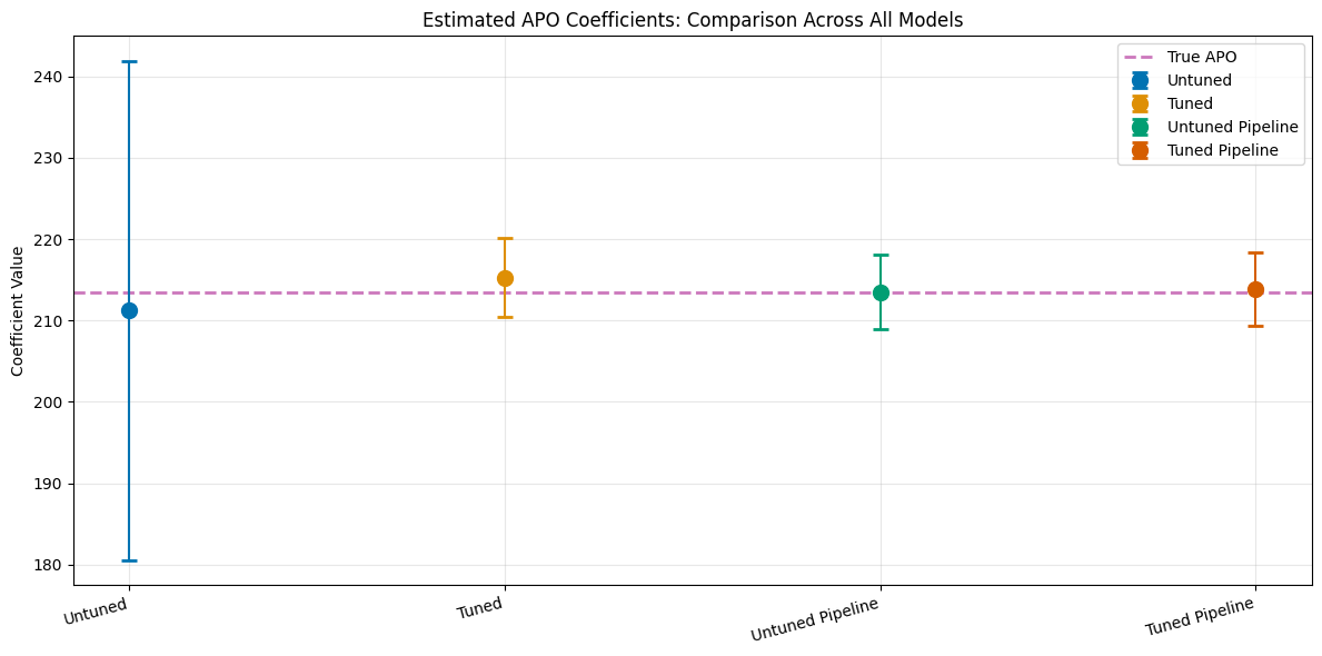
Comparison#
[23]:
ci_untuned = dml_obj_untuned.confint()
ci_tuned = dml_obj_tuned.confint()
ci_untuned_pipeline = dml_obj_untuned_pipeline.confint()
ci_tuned_pipeline = dml_obj_tuned_pipeline.confint()

# Create comparison dataframe
comparison_data = {
    'Model': ['Untuned', 'Tuned', 'Untuned Pipeline', 'Tuned Pipeline'],
    'theta': [dml_obj_untuned.coef[0], dml_obj_tuned.coef[0], dml_obj_untuned_pipeline.coef[0], dml_obj_tuned_pipeline.coef[0]],
    'se': [dml_obj_untuned.se[0], dml_obj_tuned.se[0], dml_obj_untuned_pipeline.se[0], dml_obj_tuned_pipeline.se[0]],
    'ci_lower': [ci_untuned.iloc[0, 0], ci_tuned.iloc[0, 0],
                 ci_untuned_pipeline.iloc[0, 0], ci_tuned_pipeline.iloc[0, 0]],
    'ci_upper': [ci_untuned.iloc[0, 1], ci_tuned.iloc[0, 1],
                 ci_untuned_pipeline.iloc[0, 1], ci_tuned_pipeline.iloc[0, 1]]
}
df_comparison = pd.DataFrame(comparison_data)

print(f"\nTrue APO at treatment level {treatment_lvl}: {apos[int(treatment_lvl)]:.4f}\n")
print(df_comparison.to_string(index=False))

# Create plot with all 4 models
plt.figure(figsize=(12, 6))

for i in range(len(df_comparison)):
    plt.errorbar(i, df_comparison.loc[i, 'theta'],
                 yerr=[[df_comparison.loc[i, 'theta'] - df_comparison.loc[i, 'ci_lower']],
                       [df_comparison.loc[i, 'ci_upper'] - df_comparison.loc[i, 'theta']]],
                 fmt='o', capsize=5, capthick=2, ecolor=palette[i], color=palette[i],
                 label=df_comparison.loc[i, 'Model'], markersize=10, zorder=2)

plt.axhline(y=apos[int(treatment_lvl)], color=palette[4], linestyle='--',
            linewidth=2, label='True APO', zorder=1)

plt.title('Estimated APO Coefficients: Comparison Across All Models')
plt.ylabel('Coefficient Value')
plt.xticks(range(4), df_comparison['Model'], rotation=15, ha='right')
plt.legend()
plt.grid(True, alpha=0.3)
plt.tight_layout()
plt.show()
True APO at treatment level 1.0: 213.4904

           Model      theta        se   ci_lower   ci_upper
         Untuned 211.232659 15.657431 180.544657 241.920661
           Tuned 215.273433  2.485000 210.402924 220.143943
Untuned Pipeline 213.512885  2.335125 208.936124 218.089647
  Tuned Pipeline 213.863430  2.276774 209.401035 218.325825
Detailed Tuning Result Analysis#
The tune_ml_models() method creates several Optuna Studies, which can be inspected in detail via the returned results.
The results are a list of dictionaries, which contain a corresponding DMLOptunaResult for each treatment variable on the param_names level, i.e. for each Optuna Study object a separate DMLOptunaResult is constructed.
[24]:
# Optuna results for the single treatment
print(tuning_results[0].keys())
dict_keys(['ml_g_d_lvl0', 'ml_g_d_lvl1', 'ml_m'])
In this example, we take a more detailed look in the tuning of ml_m
[25]:
print(tuning_results[0]['ml_m'])
================== DMLOptunaResult ==================
Learner name: ml_m
Params name: ml_m
Tuned: True
Best score: -0.5210215656500876
Scoring method: neg_log_loss

------------------ Best parameters    ------------------
{'stacking__final_estimator__C': 99.9143065172164,
 'stacking__lgbm__lambda_l1': 9.771463014326052,
 'stacking__lgbm__lambda_l2': 0.0013978426220758982,
 'stacking__lgbm__learning_rate': 0.0011563701553192595,
 'stacking__lgbm__min_child_samples': 30}
As we have access to the saved Optuna Study object, it is possible to access all trials and hyperparameter combinations
[26]:
ml_m_study = tuning_results[0]['ml_m'].study
ml_m_study.trials_dataframe()
[26]:
| number | value | datetime_start | datetime_complete | duration | params_stacking__final_estimator__C | params_stacking__lgbm__lambda_l1 | params_stacking__lgbm__lambda_l2 | params_stacking__lgbm__learning_rate | params_stacking__lgbm__min_child_samples | state | |
|---|---|---|---|---|---|---|---|---|---|---|---|
| 0 | 0 | -0.528553 | 2025-11-26 15:53:57.489511 | 2025-11-26 15:53:57.890548 | 0 days 00:00:00.401037 | 0.037301 | 0.498575 | 0.001738 | 0.060706 | 30 | COMPLETE |
| 1 | 1 | -0.523453 | 2025-11-26 15:53:57.891547 | 2025-11-26 15:53:58.267444 | 0 days 00:00:00.375897 | 24.451158 | 2.007596 | 0.013849 | 0.065453 | 50 | COMPLETE |
| 2 | 2 | -0.528991 | 2025-11-26 15:53:58.268406 | 2025-11-26 15:53:58.600445 | 0 days 00:00:00.332039 | 0.014914 | 1.540299 | 0.242604 | 0.030858 | 40 | COMPLETE |
| 3 | 3 | -0.521994 | 2025-11-26 15:53:58.601158 | 2025-11-26 15:53:58.929636 | 0 days 00:00:00.328478 | 43.646318 | 7.867187 | 0.004868 | 0.010726 | 20 | COMPLETE |
| 4 | 4 | -0.528075 | 2025-11-26 15:53:58.930497 | 2025-11-26 15:53:59.343117 | 0 days 00:00:00.412620 | 0.235419 | 0.636639 | 6.249970 | 0.014593 | 30 | COMPLETE |
| ... | ... | ... | ... | ... | ... | ... | ... | ... | ... | ... | ... |
| 195 | 195 | -0.521644 | 2025-11-26 15:55:14.129881 | 2025-11-26 15:55:14.449172 | 0 days 00:00:00.319291 | 97.760868 | 7.085697 | 0.001097 | 0.001008 | 30 | COMPLETE |
| 196 | 196 | -0.521990 | 2025-11-26 15:55:14.449715 | 2025-11-26 15:55:14.810118 | 0 days 00:00:00.360403 | 99.447375 | 6.005734 | 0.001353 | 0.001181 | 30 | COMPLETE |
| 197 | 197 | -0.521118 | 2025-11-26 15:55:14.810960 | 2025-11-26 15:55:15.111526 | 0 days 00:00:00.300566 | 99.675451 | 7.589184 | 0.001779 | 0.001080 | 30 | COMPLETE |
| 198 | 198 | -0.525316 | 2025-11-26 15:55:15.112415 | 2025-11-26 15:55:15.543287 | 0 days 00:00:00.430872 | 99.982456 | 0.016786 | 0.001159 | 0.001184 | 30 | COMPLETE |
| 199 | 199 | -0.521044 | 2025-11-26 15:55:15.544058 | 2025-11-26 15:55:15.826366 | 0 days 00:00:00.282308 | 80.453189 | 9.930357 | 0.001576 | 0.001073 | 30 | COMPLETE |
200 rows × 11 columns
Additionally, we can access all Optuna visualization options
[27]:
fig = optuna.visualization.plot_optimization_history(ml_m_study)
show(fig)
[28]:
fig = optuna.visualization.plot_parallel_coordinate(ml_m_study)
show(fig)
[29]:
fig = optuna.visualization.plot_param_importances(ml_m_study)
show(fig)
DoubleMLAPOS Tuning Example#
We will repeat the tuning procedure for all treatment level with the DoubleMLAPOS object. Combined DoubleML object, such as DoubleMLAPOS or DoubleMLDIDMulti just pass the tuning arguments to the underlying submodels.
[30]:
treatment_lvls = np.unique(d)
print(treatment_lvls)
[0. 1. 2. 3.]
Consequently, we are tuning \(3\) learners for each treatment level.
Untuned Model#
Again, let’s start with the untuned model. We will focus on just on the boosted trees to highlight the ideas.
[31]:
dml_apos_untuned = DoubleMLAPOS(
    dml_data,
    ml_g,
    ml_m,
    treatment_levels=treatment_lvls,
)
dml_apos_untuned.fit()
dml_apos_untuned.summary
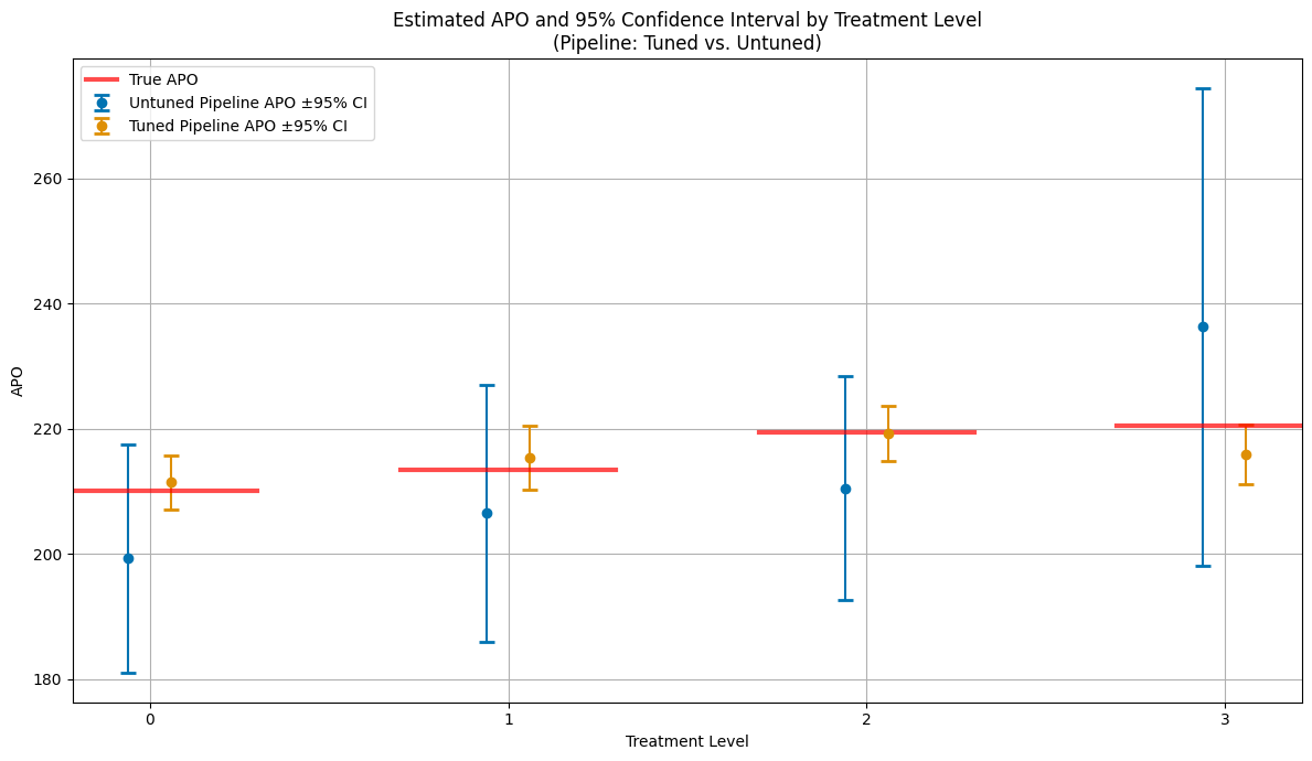
[31]:
| coef | std err | t | P>|t| | 2.5 % | 97.5 % | |
|---|---|---|---|---|---|---|
| 0.0 | 199.244627 | 9.335496 | 21.342693 | 0.0 | 180.947391 | 217.541863 |
| 1.0 | 206.488551 | 10.468016 | 19.725662 | 0.0 | 185.971617 | 227.005485 |
| 2.0 | 210.440867 | 9.128061 | 23.054279 | 0.0 | 192.550196 | 228.331538 |
| 3.0 | 236.296077 | 19.486692 | 12.126023 | 0.0 | 198.102863 | 274.489292 |
Hyperparameter Tuning#
Let’s initialize a second DoubleMLAPOS object.
[32]:
dml_apos_tuned = DoubleMLAPOS(
    dml_data,
    ml_g,
    ml_m,
    treatment_levels=treatment_lvls,
)
Again, we can directly call the tune_ml_models() method for tuning. This will take some time as each submodel is tuned.
[33]:
dml_apos_tuned.tune_ml_models(
    ml_param_space=param_space,
    optuna_settings=optuna_settings_pipeline,
)
[33]:
<doubleml.irm.apos.DoubleMLAPOS at 0x7f028a1bb4a0>
Afterwards, all hyperparameters are set for each submodel and we can proceed as usual.
[34]:
dml_apos_tuned.fit()
dml_apos_tuned.summary
[34]:
| coef | std err | t | P>|t| | 2.5 % | 97.5 % | |
|---|---|---|---|---|---|---|
| 0.0 | 211.422244 | 2.233931 | 94.641355 | 0.0 | 207.043820 | 215.800668 |
| 1.0 | 215.370889 | 2.581675 | 83.422933 | 0.0 | 210.310899 | 220.430878 |
| 2.0 | 219.233573 | 2.243180 | 97.733404 | 0.0 | 214.837022 | 223.630124 |
| 3.0 | 215.927956 | 2.442976 | 88.387268 | 0.0 | 211.139811 | 220.716100 |
[35]:
dml_apos_tuned.causal_contrast(reference_levels=[0]).summary
[35]:
| coef | std err | t | P>|t| | 2.5 % | 97.5 % | |
|---|---|---|---|---|---|---|
| 1.0 vs 0.0 | 3.948644 | 2.615180 | 1.509894 | 0.131071 | -1.177015 | 9.074303 |
| 2.0 vs 0.0 | 7.811329 | 2.375106 | 3.288833 | 0.001006 | 3.156205 | 12.466452 |
| 3.0 vs 0.0 | 4.505712 | 2.579080 | 1.747023 | 0.080633 | -0.549192 | 9.560616 |
Finally, lets compare the estimates including confidence intervals.
[36]:
# --- Plot APOs and 95% CIs for all treatment levels (tuned vs. untuned pipeline) ---

plt.figure(figsize=(12, 7))
palette = sns.color_palette("colorblind")

# Collect results for each treatment level from both models
treatment_levels_plot = np.unique(d)
n_levels = len(treatment_levels_plot)

# Prepare DataFrame for plotting
df_apo_plot = pd.DataFrame({
    'treatment_level': np.tile(treatment_levels_plot, 2),
    'APO': np.concatenate([dml_apos_untuned.coef, dml_apos_tuned.coef]),
    'ci_lower': np.concatenate([dml_apos_untuned.confint().iloc[:, 0], dml_apos_tuned.confint().iloc[:, 0]]),
    'ci_upper': np.concatenate([dml_apos_untuned.confint().iloc[:, 1], dml_apos_tuned.confint().iloc[:, 1]]),
    'Model': ['Untuned Pipeline'] * n_levels + ['Tuned Pipeline'] * n_levels
})

jitter_strength = 0.12
models = df_apo_plot['Model'].unique()
n_models = len(models)

for i, model in enumerate(models):
    df = df_apo_plot[df_apo_plot['Model'] == model]
    jitter = (i - (n_models - 1) / 2) * jitter_strength
    x_jittered = df['treatment_level'] + jitter
    plt.errorbar(
        x_jittered,
        df['APO'],
        yerr=[df['APO'] - df['ci_lower'], df['ci_upper'] - df['APO']],
        fmt='o',
        capsize=5,
        capthick=2,
        ecolor=palette[i % len(palette)],
        color=palette[i % len(palette)],
        label=f"{model} APO ±95% CI",
        zorder=2
    )

# Add true APOs as horizontal lines
x_range = plt.xlim()
total_width = x_range[1] - x_range[0]
for i, level in enumerate(treatment_levels_plot):
    line_width = 0.6
    x_center = level
    x_start = x_center - line_width/2
    x_end = x_center + line_width/2
    xmin_rel = max(0, (x_start - x_range[0]) / total_width)
    xmax_rel = min(1, (x_end - x_range[0]) / total_width)
    plt.axhline(y=apos[int(level)], color='red', linestyle='-', alpha=0.7,
                xmin=xmin_rel, xmax=xmax_rel,
                linewidth=3, label='True APO' if i == 0 else "")

plt.title('Estimated APO and 95% Confidence Interval by Treatment Level\n(Pipeline: Tuned vs. Untuned)')
plt.xlabel('Treatment Level')
plt.ylabel('APO')
plt.xticks(treatment_levels_plot)
plt.legend()
plt.grid(True)
plt.tight_layout()
plt.show()