Note
-
Download Jupyter notebook:
https://docs.doubleml.org/stable/examples/py_double_ml_did.ipynb.
Python: Difference-in-Differences#
In this example, we illustrate how the DoubleML package can be used to estimate the average treatment effect on the treated (ATT) under the conditional parallel trend assumption. The estimation is based on Chang (2020), Sant’Anna and Zhao (2020) and Zimmert et al. (2018).
In this example, we will adopt the notation of Sant’Anna and Zhao (2020).
In the whole example our treatment and time variable \(t\in\{0,1\}\) will be binary. Let \(D_i\in\{0,1\}\) denote the treatment status of unit \(i\) at time \(t=1\) (at time \(t=0\) all units are not treated) and let \(Y_{it}\) be the outcome of interest of unit \(i\) at time \(t\). Using the potential outcome notation, we can write \(Y_{it}(d)\) for the potential outcome of unit \(i\) at time \(t\) and treatment status \(d\). Further, let \(X_i\) denote a vector of pre-treatment covariates. In these difference-in-differences settings Abadie (2005) showed that the ATTE
is identified when panel data are available or under stationarity assumptions for repeated cross-sections. Further, the basic assumptions are
Parallel Trends: We have \(\mathbb{E}[Y_{i1}(0) - Y_{i0}(0)|X_i, D_i=1] = \mathbb{E}[Y_{i1}(0) - Y_{i0}(0)|X_i, D_i=0]\quad a.s.\)
Overlap: For some \(\epsilon > 0\), \(P(D_i=1) > \epsilon\) and \(P(D_i=1|X_i) \le 1-\epsilon\) a.s.
For a detailed explanation of the assumptions see e.g. Sant’Anna and Zhao (2020) or Zimmert et al. (2018).
Panel Data (Repeated Outcomes)#
At first, we will consider two-period panel data, where we observe i.i.d. data \(W_i = (Y_{i0}, Y_{i1}, D_i, X_i)\).
Data#
We will use the implemented data generating process make_did_SZ2020 to generate data according to the simulation in Sant’Anna and Zhao (2020) (Section 4.1).
In this example, we will use dgp_tpye=4, which corresponds to the misspecified settings in Sant’Anna and Zhao (2020) (other data generating processes are also available via the dgp_type parameter). In all settings the true ATTE is zero.
To specify a corresponding DoubleMLData object, we have to specify a single outcome y. For panel data, the outcome consists of the difference of
This difference will then be defined as outcome in our DoubleMLData object. The data generating process make_did_SZ2020 already specifies the outcome y accordingly.
[1]:
import numpy as np
from doubleml.datasets import make_did_SZ2020
from doubleml import DoubleMLData

np.random.seed(42)
n_obs = 1000
x, y, d = make_did_SZ2020(n_obs=n_obs, dgp_type=4, cross_sectional_data=False, return_type='array')
dml_data = DoubleMLData.from_arrays(x=x, y=y, d=d)
print(dml_data)
================== DoubleMLData Object ==================

------------------ Data summary      ------------------
Outcome variable: y
Treatment variable(s): ['d']
Covariates: ['X1', 'X2', 'X3', 'X4']
Instrument variable(s): None
No. Observations: 1000

------------------ DataFrame info    ------------------
<class 'pandas.core.frame.DataFrame'>
RangeIndex: 1000 entries, 0 to 999
Columns: 6 entries, X1 to d
dtypes: float64(6)
memory usage: 47.0 KB
ATTE Estimation#
To estimate the ATTE with panel data, we will use the DoubleMLDID class.
As for all DoubleML classes, we have to specify learners, which have to be initialized first. Here, we will just rely on a tree based method.
The learner ml_g is used to fit conditional expectations of the outcome \(\mathbb{E}[\Delta Y_i|D_i=0, X_i]\), whereas the learner ml_m will be used to estimate the propensity score \(P(D_i=1|X_i)\).
[2]:
from lightgbm import LGBMClassifier, LGBMRegressor

n_estimators = 30
ml_g = LGBMRegressor(n_estimators=n_estimators)
ml_m = LGBMClassifier(n_estimators=n_estimators)
The DoubleMLDID class can be used as any other DoubleML class.
The score is set to score='observational', since the we generated data where the treatment probability depends on the pretreatment covariates. Further, we will use in_sample_normalization=True, since normalization generally improved the results in our simulations (both score='observational' and in_sample_normalization=True are default values).
After initialization, we have to call the fit() method to estimate the nuisance elements.
[3]:
from doubleml import DoubleMLDID
dml_did = DoubleMLDID(dml_data,
                      ml_g=ml_g,
                      ml_m=ml_m,
                      score='observational',
                      in_sample_normalization=True,
                      n_folds=5)

dml_did.fit()
print(dml_did)
================== DoubleMLDID Object ==================

------------------ Data summary      ------------------
Outcome variable: y
Treatment variable(s): ['d']
Covariates: ['X1', 'X2', 'X3', 'X4']
Instrument variable(s): None
No. Observations: 1000

------------------ Score & algorithm ------------------
Score function: observational
DML algorithm: dml2

------------------ Machine learner   ------------------
Learner ml_g: LGBMRegressor(n_estimators=30)
Learner ml_m: LGBMClassifier(n_estimators=30)
Out-of-sample Performance:
Learner ml_g0 RMSE: [[11.43627032]]
Learner ml_g1 RMSE: [[11.66989604]]
Learner ml_m RMSE: [[0.48873663]]

------------------ Resampling        ------------------
No. folds: 5
No. repeated sample splits: 1
Apply cross-fitting: True

------------------ Fit summary       ------------------
       coef   std err         t     P>|t|     2.5 %    97.5 %
d  1.386988  1.827375  0.759006  0.447849 -2.194601  4.968577
As usual, confidence intervals at different levels can be obtained via
[4]:
print(dml_did.confint(level=0.90))
      5.0 %    95.0 %
d -1.618776  4.392752
Coverage Simulation#
Here, we add a small coverage simulation to highlight the difference to the linear implementation of Sant’Anna and Zhao (2020). We generate multiple datasets, estimate the ATTE and collect the results (this may take some time).
[5]:
n_rep = 200
ATTE = 0.0

ATTE_estimates = np.full((n_rep), np.nan)
coverage = np.full((n_rep), np.nan)
ci_length = np.full((n_rep), np.nan)

np.random.seed(42)
for i_rep in range(n_rep):
    if (i_rep % int(n_rep/10)) == 0:
        print(f'Iteration: {i_rep}/{n_rep}')
    dml_data = make_did_SZ2020(n_obs=n_obs, dgp_type=4, cross_sectional_data=False)

    dml_did = DoubleMLDID(dml_data, ml_g=ml_g, ml_m=ml_m, n_folds=5)
    dml_did.fit()

    ATTE_estimates[i_rep] = dml_did.coef.squeeze()
    confint = dml_did.confint(level=0.95)
    coverage [i_rep] = (confint['2.5 %'].iloc[0] <= ATTE) & (ATTE <= confint['97.5 %'].iloc[0])
    ci_length[i_rep] = confint['97.5 %'].iloc[0] - confint['2.5 %'].iloc[0]
Iteration: 0/200
Iteration: 20/200
Iteration: 40/200
Iteration: 60/200
Iteration: 80/200
Iteration: 100/200
Iteration: 120/200
Iteration: 140/200
Iteration: 160/200
Iteration: 180/200
Let us take a look at the corresponding coverage and the length of the confidence intervals.
[6]:
print(f'Coverage: {coverage.mean()}')
print(f'Average CI length: {ci_length.mean()}')
Coverage: 0.925
Average CI length: 5.32236455588136
Here, we can observe that the coverage is still valid, since we did not rely on linear learners, so the setting is not misspecified in this example.
If we know the conditional expectation is correctly specified (linear form), we can use this to obtain smaller confidence intervals but in many applications, we may want to safeguard against misspecification and use flexible models such as random forest or boosting.
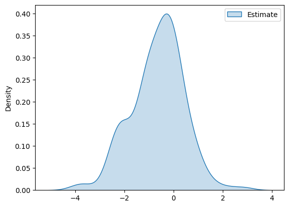
The distribution of the estimates takes the following form
[7]:
import pandas as pd
import matplotlib.pyplot as plt
import seaborn as sns

df_pa = pd.DataFrame(ATTE_estimates, columns=['Estimate'])
g = sns.kdeplot(df_pa, fill=True)
plt.show()
Repeated Cross-Sectional Data#
For repeated cross-sectional data, we assume that we observe i.i.d. data \(W_i = (Y_{i}, D_i, X_i, T_i)\).
Here \(Y_i = T_i Y_{i1} + (1-T_i)Y_{i0}\) corresponds to the outcome of unit \(i\) which is observed at time \(T_i\).
Data#
As for panel data, we will use the implemented data generating process make_did_SZ2020 to generate data according to the simulation in Sant’Anna and Zhao (2020) (Section 4.2).
In this example, we will use dgp_tpye=4, which corresponds to the misspecified settings in Sant’Anna and Zhao (2020) (other data generating processes are also available via the dgp_type parameter). In all settings the true ATTE is zero.
In contrast to other DoubleMLData objects, we have to specify which column corresponds to our time variable \(T\).
The time variable can be simply set via the argument t.
[8]:
import numpy as np
from doubleml.datasets import make_did_SZ2020
from doubleml import DoubleMLData

np.random.seed(42)
n_obs = 1000
x, y, d, t = make_did_SZ2020(n_obs=n_obs, dgp_type=4, cross_sectional_data=True, return_type='array')
dml_data = DoubleMLData.from_arrays(x=x, y=y, d=d, t=t)
print(dml_data)
================== DoubleMLData Object ==================

------------------ Data summary      ------------------
Outcome variable: y
Treatment variable(s): ['d']
Covariates: ['X1', 'X2', 'X3', 'X4']
Instrument variable(s): None
Time variable: t
No. Observations: 1000

------------------ DataFrame info    ------------------
<class 'pandas.core.frame.DataFrame'>
RangeIndex: 1000 entries, 0 to 999
Columns: 7 entries, X1 to t
dtypes: float64(7)
memory usage: 54.8 KB
ATTE Estimation#
To estimate the ATTE with panel data, we will use the DoubleMLDIDCS class.
As for all DoubleML classes, we have to specify learners, which have to be initialized first. Here, we will just rely on a tree based method.
The learner ml_g is used to fit conditional expectations of the outcome \(\mathbb{E}[\Delta Y_i| D_i=d, T_i =t, X_i]\) for all combinations of \(d,t\in\{0,1\}\), whereas the learner ml_m will be used to estimate the propensity score \(P(D_i=1|X_i)\).
[9]:
from lightgbm import LGBMClassifier, LGBMRegressor

n_estimators = 30
ml_g = LGBMRegressor(n_estimators=n_estimators)
ml_m = LGBMClassifier(n_estimators=n_estimators)
The DoubleMLDIDCS class can be used as any other DoubleML class.
The score is set to score='observational', since the we generated data where the treatment probability depends on the pretreatment covariates. Further, we will use in_sample_normalization=True, since normalization generally improved the results in our simulations (both score='observational' and in_sample_normalization=True are default values).
After initialization, we have to call the fit() method to estimate the nuisance elements.
[10]:
from doubleml import DoubleMLDIDCS
dml_did = DoubleMLDIDCS(dml_data,
                        ml_g=ml_g,
                        ml_m=ml_m,
                        score='observational',
                        in_sample_normalization=True,
                        n_folds=5)

dml_did.fit()
print(dml_did)
================== DoubleMLDIDCS Object ==================

------------------ Data summary      ------------------
Outcome variable: y
Treatment variable(s): ['d']
Covariates: ['X1', 'X2', 'X3', 'X4']
Instrument variable(s): None
Time variable: t
No. Observations: 1000

------------------ Score & algorithm ------------------
Score function: observational
DML algorithm: dml2

------------------ Machine learner   ------------------
Learner ml_g: LGBMRegressor(n_estimators=30)
Learner ml_m: LGBMClassifier(n_estimators=30)
Out-of-sample Performance:
Learner ml_g_d0_t0 RMSE: [[15.02897287]]
Learner ml_g_d0_t1 RMSE: [[26.5602727]]
Learner ml_g_d1_t0 RMSE: [[27.62403053]]
Learner ml_g_d1_t1 RMSE: [[44.06834315]]
Learner ml_m RMSE: [[0.47761563]]

------------------ Resampling        ------------------
No. folds: 5
No. repeated sample splits: 1
Apply cross-fitting: True

------------------ Fit summary       ------------------
       coef   std err         t     P>|t|     2.5 %     97.5 %
d  5.096741  5.225034  0.975447  0.329339 -5.144137  15.337619
As usual, confidence intervals at different levels can be obtained via
[11]:
print(dml_did.confint(level=0.90))
      5.0 %     95.0 %
d -3.497674  13.691157
Coverage Simulation#
Again, we add a small coverage simulation to highlight the difference to the linear implementation of Sant’Anna and Zhao (2020). We generate multiple datasets, estimate the ATTE and collect the results (this may take some time).
[12]:
n_rep = 200
ATTE = 0.0

ATTE_estimates = np.full((n_rep), np.nan)
coverage = np.full((n_rep), np.nan)
ci_length = np.full((n_rep), np.nan)

np.random.seed(42)
for i_rep in range(n_rep):
    if (i_rep % int(n_rep/10)) == 0:
        print(f'Iteration: {i_rep}/{n_rep}')
    dml_data = make_did_SZ2020(n_obs=n_obs, dgp_type=4, cross_sectional_data=True)

    dml_did = DoubleMLDIDCS(dml_data, ml_g=ml_g, ml_m=ml_m, n_folds=5)
    dml_did.fit()

    ATTE_estimates[i_rep] = dml_did.coef.squeeze()
    confint = dml_did.confint(level=0.95)
    coverage [i_rep] = (confint['2.5 %'].iloc[0] <= ATTE) & (ATTE <= confint['97.5 %'].iloc[0])
    ci_length[i_rep] = confint['97.5 %'].iloc[0] - confint['2.5 %'].iloc[0]
Iteration: 0/200
Iteration: 20/200
Iteration: 40/200
Iteration: 60/200
Iteration: 80/200
Iteration: 100/200
Iteration: 120/200
Iteration: 140/200
Iteration: 160/200
Iteration: 180/200
Let us take a look at the corresponding coverage and the length of the confidence intervals.
[13]:
print(f'Coverage: {coverage.mean()}')
print(f'Average CI length: {ci_length.mean()}')
Coverage: 0.94
Average CI length: 23.34858240261807
As for panel data the coverage is still valid, since we did not rely on linear learners, so the setting is not misspecified in this example.
If we know the conditional expectation is correctly specified (linear form), we can use this to obtain smaller confidence intervals but in many applications, we may want to safeguard against misspecification and use flexible models such as random forest or boosting.
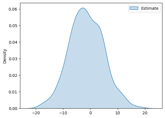
The distribution of the estimates takes the following form
[14]:
import pandas as pd
import matplotlib.pyplot as plt
import seaborn as sns

df_pa = pd.DataFrame(ATTE_estimates, columns=['Estimate'])
g = sns.kdeplot(df_pa, fill=True)
plt.show()