Note

https://docs.doubleml.org/stable/examples/py_double_ml_plpr.ipynb

Python: Static Panel Models with Fixed Effects#

In this example, we illustrate how the DoubleML package can be used to estimate treatment effects for static panel models with fixed effects in a partially linear panel regression DoubleMLPLPR model. The model is based on Clarke and Polselli (2025).

[1]:

import optuna
import numpy as np
import pandas as pd
import matplotlib.pyplot as plt
import seaborn as sns

from sklearn.base import clone
from sklearn.preprocessing import StandardScaler
from sklearn.preprocessing import PolynomialFeatures
from sklearn.compose import ColumnTransformer
from sklearn.pipeline import make_pipeline
from sklearn.base import BaseEstimator, TransformerMixin
from sklearn.linear_model import LassoCV
from lightgbm import LGBMRegressor

from doubleml.data import DoubleMLPanelData
from doubleml.plm.datasets import make_plpr_CP2025
from doubleml import DoubleMLPLPR

import warnings
warnings.filterwarnings("ignore")

Data#

We will use the implemented data generating process make_plpr_CP2025 to generate data similar to the simulation in Clarke and Polselli (2025). For exposition, we use the simple linear dgp_type="dgp1", with 150 units, 10 time periods per unit, and a true treatment effect of theta=0.5.

We set time_type="int" such that the time variable values will be integers. It’s also possible to use "float" or "datetime" time variables with DoubleMLPLPR.

[2]:

np.random.seed(123)
data = make_plpr_CP2025(num_id=150, num_t=10, dim_x=30, theta=0.5, dgp_type="dgp1", time_type="int")
data.head()

[2]:

	id	time	y	d	x1	x2	x3	x4	x5	x6	...	x21	x22	x23	x24	x25	x26	x27	x28	x29	x30
0	1	1	-1.290479	0.908307	1.710715	-1.853675	-1.473907	1.366514	-0.322024	2.944020	...	-1.828362	-3.010547	-0.840202	-3.085159	1.169952	-0.954107	-3.925198	-0.779510	-0.430700	1.004298
1	1	2	-2.850646	-1.316777	-0.325043	4.178599	-1.159857	-0.139527	-0.230115	-0.631976	...	-0.724172	-0.421045	-2.012480	-2.081784	-2.734123	-0.879470	-2.141218	4.598401	-4.222797	-2.523024
2	1	3	-4.338502	-1.756120	-0.897590	1.505972	-0.925189	1.511500	-2.206561	0.132579	...	1.766109	-2.252858	-2.919826	-1.974066	-0.773881	0.244633	-1.727550	1.665467	0.562291	-1.553616
3	1	4	-2.713236	0.934866	1.987849	2.596228	-0.220666	-0.480717	-3.966273	-0.911226	...	0.856124	0.727759	-0.501579	1.077504	2.268052	-3.821422	1.629055	-0.220834	-1.185091	-5.462884
4	1	5	-5.782997	-4.357881	-3.086559	3.796975	-1.539641	-2.425617	-1.020599	-1.666200	...	2.617215	-1.231835	-0.891350	0.246981	2.489642	0.319735	-2.810366	0.585826	3.643749	0.147147

5 rows × 34 columns

To create a corresponding DoubleMLPanelData object, we need to set static_panel=True and specify id_col and time_col columns.

[3]:

data_obj = DoubleMLPanelData(data, y_col="y", d_cols="d", t_col="time", id_col="id", static_panel=True)

Model#

The partially linear panel regression (PLPR) model extends the partially linear model to panel data by introducing fixed effects \(\alpha_i^*\).

The PLPR model takes the form

\[\begin{split}\begin{align*} Y_{it} &= \theta_0 D_{it} + g_1(X_{it}) + \alpha_i^* + U_{it}, \\ D_{it} &= m_1(X_{it}) + \gamma_i + V_{it}, \end{align*}\end{split}\]

where

\(Y_{it}\) outcome, \(D_{it}\) treatment, \(X_{it}\) covariates, \(\theta_0\) causal treatment effect
\(g_1\) and \(m_1\) nuisance functions
\(\alpha_i^*\), \(\gamma_i\) unobserved individual heterogeneity, correlated with covariates
\(U_{it}\), \(V_{it}\) error terms

Further note \(\mathbb{E}[U_{it} \mid D_{it}, X_{it}, \alpha_i^*] = 0\) and \(\mathbb{E}[V_{it} \mid X_{it}, \gamma_i]=0\), but \(\mathbb{E}[\alpha_i^* \mid D_{it}, X_{it}] \neq 0\).

Alternatively we can write the partialling-out PLPR as

\[\begin{split}\begin{align*} Y_{it} &= \theta_0 V_{it} + \ell_1(X_{it}) + \alpha_i + U_{it}, \\ V_{it} &= D_{it} - m_1(X_{it}) - \gamma_i, \end{align*}\end{split}\]

with nuisance function \(\ell_1\) and fixed effect \(\alpha_i\).

Assumptions#

Define \(\xi_i\) as time-invariant heterogeneity terms influencing outcome and treatment and \(L_{t-1}(W_i) = \{ W_{i1}, \dots, W_{it-1} \}\) as lags of a random variable \(W_{it}\) at wave \(t\).

No feedback to predictors

\[X_{it} \perp L_{t-1} (Y_i, D_i) \mid L_{t-1} (X_i), \xi_i\]
Static panel

\[Y_{it}, D_{it} \perp L_{t-1} (Y_i, X_i, D_i) \mid X_{it}, \xi_i\]
Selection on observables and omitted time-invariant variables

\[Y_{it} (.) \perp D_{it} \mid X_{it}, \xi_i\]
Homogeneity and linearity of the treatment effect

\[\mathbb{E} [Y_{it}(d) - Y_{it}(0) \mid X_{it}, \xi_i] = d \theta_0\]
Additive Separability

\[\begin{split}\begin{align*} \mathbb{E} [Y_{it}(0) \mid X_{it}, \xi_i] &= g_1(X_{it}) + \alpha^*_i \quad \text{where } \alpha^*_i = \alpha^*(\xi_i), \\ \mathbb{E} [D_{it} \mid X_{it}, \xi_i] &= m_1(X_{it}) + \gamma_i \quad \text{where } \gamma_i = \gamma(\xi_i) \end{align*}\end{split}\]

For more information, see Clarke and Polselli (2025).

To estimate the causal effect, we can create a DoubleMLPLPR object. The model described in Clarke and Polselli (2025) uses block-k-fold cross-fitting, where the entire time series of the sampled unit is allocated to one fold to allow for possible serial correlation within each unit which is common with panel data. Furthermore, cluster robust standard error are employed. DoubleMLPLPR implements both aspects by using id_col as the cluster variable.

Estimation Approaches#

Clarke and Polselli (2025) describes multiple estimation approaches, which can be set with the approach parameter. Depending on the type of approach, different data transformations are performed along the way.

Correlated Random Effects#

The correlated random effects (cre) approaches includes the a general approach (cre_general) and an approach relying on normality assumptions (cre_normal).

`cre_general`#

The cre_general approach:

Learning \(\ell_1\) from \(\{ Y_{it}, X_{it}, \bar{X}_i : t=1,\dots, T \}_{i=1}^N\).
First learning \(\tilde{m}_1\) from \(\{ D_{it}, X_{it}, \bar{X}_i : t=1,\dots, T \}_{i=1}^N\), with predictions \(\hat{m}_{1,it} = \tilde{m}_1 (X_{it}, \bar{X}_i)\)
- Calculate \(\hat{\bar{m}}_i = T^{-1} \sum_{t=1}^T \hat{m}_{1,it}\),
- Calculate final nuisance part as \(\hat{m}^*_1 (X_{it}, \bar{X}_i, \bar{D}_i) = \hat{m}_{1,it} + \bar{D}_i - \hat{\bar{m}}_i\).

[4]:

learner = LassoCV()
ml_l = clone(learner)
ml_m = clone(learner)

dml_plpr_cre_general = DoubleMLPLPR(data_obj, ml_l=ml_l, ml_m=ml_m, approach="cre_general", n_folds=5)

We can look at the the transformed data using the data_transform property after the DoubleMLPLPR object was created.

[5]:

dml_plpr_cre_general.data_transform.data.head()

[5]:

	id	time	y	d	x1	x2	x3	x4	x5	x6	...	x21_mean	x22_mean	x23_mean	x24_mean	x25_mean	x26_mean	x27_mean	x28_mean	x29_mean	x30_mean
0	1	1	-1.290479	0.908307	1.710715	-1.853675	-1.473907	1.366514	-0.322024	2.944020	...	1.24018	-0.52821	-0.734145	0.227494	1.164763	0.412979	-1.272608	0.459816	-0.829863	-1.145189
1	1	2	-2.850646	-1.316777	-0.325043	4.178599	-1.159857	-0.139527	-0.230115	-0.631976	...	1.24018	-0.52821	-0.734145	0.227494	1.164763	0.412979	-1.272608	0.459816	-0.829863	-1.145189
2	1	3	-4.338502	-1.756120	-0.897590	1.505972	-0.925189	1.511500	-2.206561	0.132579	...	1.24018	-0.52821	-0.734145	0.227494	1.164763	0.412979	-1.272608	0.459816	-0.829863	-1.145189
3	1	4	-2.713236	0.934866	1.987849	2.596228	-0.220666	-0.480717	-3.966273	-0.911226	...	1.24018	-0.52821	-0.734145	0.227494	1.164763	0.412979	-1.272608	0.459816	-0.829863	-1.145189
4	1	5	-5.782997	-4.357881	-3.086559	3.796975	-1.539641	-2.425617	-1.020599	-1.666200	...	1.24018	-0.52821	-0.734145	0.227494	1.164763	0.412979	-1.272608	0.459816	-0.829863	-1.145189

5 rows × 64 columns

We can see that the covariates inlcude the original \(X_{it}\) and additionally the unit mean \(\bar{X}_i\).

After fitting the model, we can print the DoubleMLPLPR object. The data summary corresponds to the transformed data. Additional Information at the end also includes a pre-transformation data summary.

[6]:

dml_plpr_cre_general.fit()
print(dml_plpr_cre_general)

================== DoubleMLPLPR Object ==================

------------------ Data Summary      ------------------
Outcome variable: y
Treatment variable(s): ['d']
Covariates: ['x1', 'x2', 'x3', 'x4', 'x5', 'x6', 'x7', 'x8', 'x9', 'x10', 'x11', 'x12', 'x13', 'x14', 'x15', 'x16', 'x17', 'x18', 'x19', 'x20', 'x21', 'x22', 'x23', 'x24', 'x25', 'x26', 'x27', 'x28', 'x29', 'x30', 'x1_mean', 'x2_mean', 'x3_mean', 'x4_mean', 'x5_mean', 'x6_mean', 'x7_mean', 'x8_mean', 'x9_mean', 'x10_mean', 'x11_mean', 'x12_mean', 'x13_mean', 'x14_mean', 'x15_mean', 'x16_mean', 'x17_mean', 'x18_mean', 'x19_mean', 'x20_mean', 'x21_mean', 'x22_mean', 'x23_mean', 'x24_mean', 'x25_mean', 'x26_mean', 'x27_mean', 'x28_mean', 'x29_mean', 'x30_mean']
Instrument variable(s): None
Time variable: time
Id variable: id
Static panel data: True
No. Unique Ids: 150
No. Observations: 1500

------------------ Score & Algorithm ------------------
Score function: partialling out
Static panel model approach: cre_general

------------------ Machine Learner   ------------------
Learner ml_l: LassoCV()
Learner ml_m: LassoCV()
Out-of-sample Performance:
Regression:
Learner ml_l RMSE: [[1.8336022]]
Learner ml_m RMSE: [[0.99534683]]

------------------ Resampling        ------------------
No. folds per cluster: 5
No. folds: 5
No. repeated sample splits: 1

------------------ Fit Summary       ------------------
       coef   std err          t         P>|t|     2.5 %    97.5 %
d  0.490173  0.026161  18.737077  2.468215e-78  0.438899  0.541447

------------------ Additional Information -------------
Cluster variable(s): ['id']

Pre-Transformation Data Summary:
Outcome variable: y
Treatment variable(s): ['d']
Covariates: ['x1', 'x2', 'x3', 'x4', 'x5', 'x6', 'x7', 'x8', 'x9', 'x10', 'x11', 'x12', 'x13', 'x14', 'x15', 'x16', 'x17', 'x18', 'x19', 'x20', 'x21', 'x22', 'x23', 'x24', 'x25', 'x26', 'x27', 'x28', 'x29', 'x30']
No. Observations: 1500

`cre_normal`#

The cre_normal approach:

Under the assumption that the conditional distribution \(D_{i1}, \dots, D_{iT} \mid X_{i1}, \dots X_{iT}\) is multivariate normal (see Clarke and Polselli (2025) for further details):

Learn \(\ell_1\) from \(\{ Y_{it}, X_{it}, \bar{X}_i : t=1,\dots, T \}_{i=1}^N\),
Learn \(m^*_{1}\) from \(\{ D_{it}, X_{it}, \bar{X}_i, \bar{D}_i: t=1,\dots, T \}_{i=1}^N\).

[7]:

dml_plpr_cre_normal = DoubleMLPLPR(data_obj, ml_l=ml_l, ml_m=ml_m, approach="cre_normal", n_folds=5)
dml_plpr_cre_normal.fit()
print(dml_plpr_cre_normal.summary)

       coef   std err          t         P>|t|    2.5 %    97.5 %
d  0.505807  0.027168  18.617927  2.299468e-77  0.45256  0.559055

The cre_normal approach uses additionally inlcudes \(\bar{D}_i\) in the treatment nuisance estimation. The corresponding data can be assesses by the d_mean property.

[8]:

dml_plpr_cre_normal.d_mean

[8]:

array([[-0.94278854],
       [-0.94278854],
       [-0.94278854],
       ...,
       [ 0.15320478],
       [ 0.15320478],
       [ 0.15320478]], shape=(1500, 1))

Transformation Approaches#

The transformation approaches include first differences (fd_exact) and within-group (wg_approx) transformations.

`fd_exact`#

Consider first differences (FD) transformation (fd_exact) \(Q(Y_{it})= Y_{it} - Y_{it-1}\), under the assumptions from above, Clarke and Polselli (2025) show that \(\mathbb{E}[Y_{it}-Y_{it-1} | X_{it-1},X_{it}] =\Delta \ell_1 (X_{it-1}, X_{it})\) and \(\mathbb{E}[D_{it}-D_{it-1} | X_{it-1},X_{it}] =\Delta m_1 (X_{it-1}, X_{it})\). Therefore, the transformed nuisance function can be learnt as

\(\Delta \ell_1 (X_{it-1}, X_{it})\) from \(\{ Y_{it}-Y_{it-1}, X_{it-1}, X_{it} : t=2, \dots , T \}_{i=1}^N\),
\(\Delta m_1 (X_{it-1}, X_{it})\) from \(\{ D_{it}-D_{it-1}, X_{it-1}, X_{it} : t=2, \dots , T \}_{i=1}^N\).

[9]:

dml_plpr_fd_exact = DoubleMLPLPR(data_obj, ml_l=ml_l, ml_m=ml_m, approach="fd_exact", n_folds=5)
dml_plpr_fd_exact.data_transform.data.head()

[9]:

	id	time	y_diff	d_diff	x1	x2	x3	x4	x5	x6	...	x21_lag	x22_lag	x23_lag	x24_lag	x25_lag	x26_lag	x27_lag	x28_lag	x29_lag	x30_lag
0	1	2	-1.560167	-2.225084	-0.325043	4.178599	-1.159857	-0.139527	-0.230115	-0.631976	...	-1.828362	-3.010547	-0.840202	-3.085159	1.169952	-0.954107	-3.925198	-0.779510	-0.430700	1.004298
1	1	3	-1.487856	-0.439343	-0.897590	1.505972	-0.925189	1.511500	-2.206561	0.132579	...	-0.724172	-0.421045	-2.012480	-2.081784	-2.734123	-0.879470	-2.141218	4.598401	-4.222797	-2.523024
2	1	4	1.625266	2.690986	1.987849	2.596228	-0.220666	-0.480717	-3.966273	-0.911226	...	1.766109	-2.252858	-2.919826	-1.974066	-0.773881	0.244633	-1.727550	1.665467	0.562291	-1.553616
3	1	5	-3.069761	-5.292747	-3.086559	3.796975	-1.539641	-2.425617	-1.020599	-1.666200	...	0.856124	0.727759	-0.501579	1.077504	2.268052	-3.821422	1.629055	-0.220834	-1.185091	-5.462884
4	1	6	-1.094799	0.551051	0.289315	-2.823134	-3.137179	-1.425923	-0.730116	0.232687	...	2.617215	-1.231835	-0.891350	0.246981	2.489642	0.319735	-2.810366	0.585826	3.643749	0.147147

5 rows × 64 columns

We see that the outcome and treatment variables are now labeled y_diff and d_diff to indicate the first-difference transformation. Moreover, lagged covariates \(X_{it-1}\) are added and rows for the first time period are dropped.

[10]:

dml_plpr_fd_exact.fit()
print(dml_plpr_fd_exact.summary)

            coef   std err          t         P>|t|     2.5 %    97.5 %
d_diff  0.511822  0.032746  15.630162  4.536510e-55  0.447641  0.576002

`wg_approx`#

For within-group (WG) transformation (wg_approx) \(Q(X_{it})= X_{it} - \bar{X}_{i}\), where \(\bar{X}_{i} = T^{-1} \sum_{t=1}^T X_{it}\), approximate the model as

\[\begin{split}\begin{align*} Q(Y_{it}) &\approx \theta_0 Q(D_{it}) + g_1 (Q(X_{it})) + Q(U_{it}), \\ Q(D_{it}) &\approx m_1 (Q(X_{it})) + Q(V_{it}). \end{align*}\end{split}\]

Similarly for the partialling-out PLPR

\[Q(Y_{it}) \approx \theta_0 Q(V_{it}) + \ell_1 (Q(X_{it})) + Q(U_{it}).\]

\(\ell_1\) can be learnt from transformed data \(\{ Q(Y_{it}), Q(X_{it}) : t=1,\dots,T \}_{i=1}^N\),
\(m_1\) can be learnt from transformed data \(\{ Q(D_{it}), Q(X_{it}) : t=1,\dots,T \}_{i=1}^N\).

[11]:

dml_plpr_wg_approx = DoubleMLPLPR(data_obj, ml_l=ml_l, ml_m=ml_m, approach="wg_approx", n_folds=5)
dml_plpr_wg_approx.data_transform.data.head()

[11]:

	id	time	y_demean	d_demean	x1_demean	x2_demean	x3_demean	x4_demean	x5_demean	x6_demean	...	x21_demean	x22_demean	x23_demean	x24_demean	x25_demean	x26_demean	x27_demean	x28_demean	x29_demean	x30_demean
0	1	1	1.543571	1.760660	2.207607	-2.039516	-0.642847	1.014204	0.384166	1.826013	...	-3.162933	-2.475942	0.000728	-3.344219	0.082829	-1.351303	-2.670511	-1.275344	0.407596	2.187878
1	1	2	-0.016596	-0.464424	0.171849	3.992759	-0.328797	-0.491837	0.476074	-1.749982	...	-2.058743	0.113560	-1.171550	-2.340844	-3.821246	-1.276666	-0.886531	4.102567	-3.384501	-1.339444
2	1	3	-1.504452	-0.903767	-0.400698	1.320131	-0.094129	1.159190	-1.500371	-0.985427	...	0.431538	-1.718253	-2.078895	-2.233126	-1.861004	-0.152563	-0.472863	1.169632	1.400587	-0.370036
3	1	4	0.120814	1.787219	2.484741	2.410387	0.610394	-0.833027	-3.260084	-2.029232	...	-0.478447	1.262364	0.339352	0.818443	1.180930	-4.218618	2.883741	-0.716668	-0.346795	-4.279304
4	1	5	-2.948947	-3.505528	-2.589667	3.611134	-0.708582	-2.777927	-0.314410	-2.784206	...	1.282645	-0.697230	-0.050420	-0.012080	1.402519	-0.077461	-1.555679	0.089991	4.482045	1.330727

5 rows × 34 columns

We see that the outcome, treatment and covariate variables are now labeled y_deman, d_deman, xi_deman to indicate the within-group transformations.

[12]:

dml_plpr_wg_approx.fit()
print(dml_plpr_wg_approx.summary)

              coef   std err          t         P>|t|     2.5 %    97.5 %
d_demean  0.495323  0.025841  19.167824  6.872435e-82  0.444675  0.545972

For the simple linear data generating process dgp_type="dgp1", we can see that all approaches lead to estimated close the true effect of theta=0.5.

The data_original property additionally includes the original data before any transformation was applied.

[13]:

dml_plpr_wg_approx.data_original.data.head()

[13]:

	id	time	y	d	x1	x2	x3	x4	x5	x6	...	x21	x22	x23	x24	x25	x26	x27	x28	x29	x30
0	1	1	-1.290479	0.908307	1.710715	-1.853675	-1.473907	1.366514	-0.322024	2.944020	...	-1.828362	-3.010547	-0.840202	-3.085159	1.169952	-0.954107	-3.925198	-0.779510	-0.430700	1.004298
1	1	2	-2.850646	-1.316777	-0.325043	4.178599	-1.159857	-0.139527	-0.230115	-0.631976	...	-0.724172	-0.421045	-2.012480	-2.081784	-2.734123	-0.879470	-2.141218	4.598401	-4.222797	-2.523024
2	1	3	-4.338502	-1.756120	-0.897590	1.505972	-0.925189	1.511500	-2.206561	0.132579	...	1.766109	-2.252858	-2.919826	-1.974066	-0.773881	0.244633	-1.727550	1.665467	0.562291	-1.553616
3	1	4	-2.713236	0.934866	1.987849	2.596228	-0.220666	-0.480717	-3.966273	-0.911226	...	0.856124	0.727759	-0.501579	1.077504	2.268052	-3.821422	1.629055	-0.220834	-1.185091	-5.462884
4	1	5	-5.782997	-4.357881	-3.086559	3.796975	-1.539641	-2.425617	-1.020599	-1.666200	...	2.617215	-1.231835	-0.891350	0.246981	2.489642	0.319735	-2.810366	0.585826	3.643749	0.147147

5 rows × 34 columns

Hyperparameter tuning#

In this section we will use the tune_ml_models() method to tune hyperparameters using the Optuna package. More details can found in the Python: Hyperparametertuning with Optuna example notebook.

As an example, we use LightGBM regressors and compare the estimates for the different static panel model approaches, when applied to the non-linear and discontinuous dgp3.

[31]:

dim_x = 30
theta = 0.5

np.random.seed(11)
data_tune = make_plpr_CP2025(num_id=4000, num_t=10, dim_x=dim_x, theta=theta, dgp_type="dgp3")
dml_data_tune = DoubleMLPanelData(data_tune, y_col="y", d_cols="d", t_col="time", id_col="id", static_panel=True)
ml_boost = LGBMRegressor(random_state=314, verbose=-1)

[32]:

# parameter space for both ml models
def ml_params(trial):
    return {
        "n_estimators": 100,
        "learning_rate": trial.suggest_float("learning_rate", 0.1, 0.4, log=True),
        "max_depth": trial.suggest_int("max_depth", 2, 10),
        "min_child_samples": trial.suggest_int("min_child_samples", 1, 5),
        "reg_lambda": trial.suggest_float("reg_lambda", 1e-2, 5, log=True),
    }

param_space = {
    "ml_l": ml_params,
    "ml_m": ml_params
}

optuna_settings = {
    "n_trials": 100,
    "show_progress_bar": True,
    "verbosity": optuna.logging.WARNING,  # Suppress Optuna logs
}

[33]:

plpr_tune_cre_general = DoubleMLPLPR(dml_data_tune, clone(ml_boost), clone(ml_boost), approach="cre_general", n_folds=5)

plpr_tune_cre_general.tune_ml_models(
    ml_param_space=param_space,
    optuna_settings=optuna_settings,
)

plpr_tune_cre_general.fit()
plpr_tune_cre_general.summary

[33]:

	coef	std err	t	P>\|t\|	2.5 %	97.5 %
d	0.50256	0.008025	62.620517	0.0	0.48683	0.518289

0.509102

[34]:

plpr_tune_cre_normal = DoubleMLPLPR(dml_data_tune, clone(ml_boost), clone(ml_boost), approach="cre_normal", n_folds=5)

plpr_tune_cre_normal.tune_ml_models(
    ml_param_space=param_space,
    optuna_settings=optuna_settings,
)

plpr_tune_cre_normal.fit()
plpr_tune_cre_normal.summary

[34]:

	coef	std err	t	P>\|t\|	2.5 %	97.5 %
d	0.461759	0.010308	44.796854	0.0	0.441556	0.481962

[35]:

plpr_tune_fd = DoubleMLPLPR(dml_data_tune, clone(ml_boost), clone(ml_boost), approach="fd_exact", n_folds=5)

plpr_tune_fd.tune_ml_models(
    ml_param_space=param_space,
    optuna_settings=optuna_settings,
)

plpr_tune_fd.fit()
plpr_tune_fd.summary

[35]:

	coef	std err	t	P>\|t\|	2.5 %	97.5 %
d_diff	0.545698	0.008928	61.12373	0.0	0.5282	0.563196

[36]:

plpr_tune_wg = DoubleMLPLPR(dml_data_tune, clone(ml_boost), clone(ml_boost), approach="wg_approx", n_folds=5)

plpr_tune_wg.tune_ml_models(
    ml_param_space=param_space,
    optuna_settings=optuna_settings,
)

plpr_tune_wg.fit()
plpr_tune_wg.summary

[36]:

	coef	std err	t	P>\|t\|	2.5 %	97.5 %
d_demean	1.1365	0.005177	219.547846	0.0	1.126354	1.146646

[37]:

palette = sns.color_palette("colorblind")

ci_cre_general = plpr_tune_cre_general.confint()
ci_cre_normal = plpr_tune_cre_normal.confint()
ci_fd = plpr_tune_fd.confint()
ci_wg = plpr_tune_wg.confint()

comparison_data = {
    "Model": ["cre_general", "cre_normal", "fd_exact", "wg_approx"],
    "theta": [plpr_tune_cre_general.coef[0], plpr_tune_cre_normal.coef[0], plpr_tune_fd.coef[0], plpr_tune_wg.coef[0]],
    "se": [plpr_tune_cre_general.se[0], plpr_tune_cre_normal.se[0], plpr_tune_fd.se[0], plpr_tune_wg.se[0]],
    "ci_lower": [ci_cre_general.iloc[0, 0], ci_cre_normal.iloc[0, 0], ci_fd.iloc[0, 0], ci_wg.iloc[0, 0]],
    "ci_upper": [ci_cre_general.iloc[0, 1], ci_cre_normal.iloc[0, 1], ci_fd.iloc[0, 1], ci_wg.iloc[0, 1]]
}
df_comparison = pd.DataFrame(comparison_data)

print(f"True treatment effect: {theta}\n")
print(df_comparison.to_string(index=False))

# Create comparison plot
plt.figure(figsize=(12, 6))

for i in range(len(df_comparison)):
    plt.errorbar(i, df_comparison.loc[i, "theta"],
                 yerr=[[df_comparison.loc[i, "theta"] - df_comparison.loc[i, "ci_lower"]],
                       [df_comparison.loc[i, "ci_upper"] - df_comparison.loc[i, "theta"]]],
                 fmt='o', capsize=5, capthick=2, ecolor=palette[i], color=palette[i],
                 label=df_comparison.loc[i, "Model"], markersize=10, zorder=2)
plt.axhline(y=theta, color=palette[4], linestyle='--',
            linewidth=2, label="True effect", zorder=1)

plt.title("Comparison across DoubleMLPLPR approaches")
plt.ylabel("Coefficient Value")
plt.xticks(range(4), df_comparison["Model"], rotation=15, ha="right")
plt.legend()
plt.grid(True, alpha=0.3)
plt.tight_layout()
plt.show()

True treatment effect: 0.5

      Model    theta       se  ci_lower  ci_upper
cre_general 0.502560 0.008025  0.486830  0.518289
 cre_normal 0.461759 0.010308  0.441556  0.481962
   fd_exact 0.545698 0.008928  0.528200  0.563196
  wg_approx 1.136500 0.005177  1.126354  1.146646

../_images/examples_py_double_ml_plpr_65_1.png

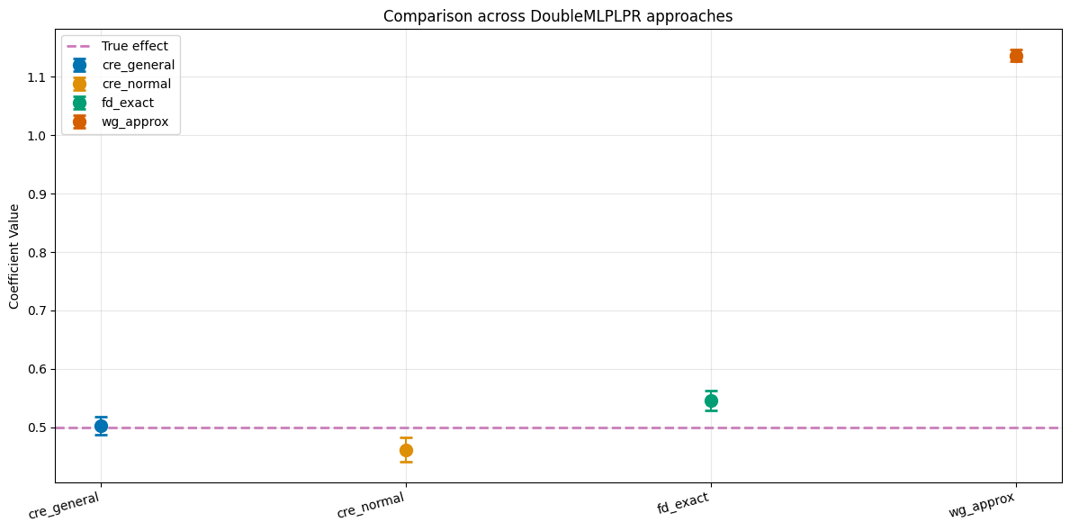
We again see that the wg_approx leads to a biased estimate in the non-linear and discontinuous dgp3 setting. The approaches cre_general, cre_normal, fd_exact, in combination with LightGBM regressors, tuned using the Optuna package, lead to estimate close to the true treatment effect.

This is line with the simulation results in Clarke and Polselli (2025), albeit only for only one dataset in this example.

Python: Static Panel Models with Fixed Effects#

Data#

Model#

Assumptions#

Estimation Approaches#

Correlated Random Effects#

cre_general#

cre_normal#

Transformation Approaches#

fd_exact#

wg_approx#

Feature preprocessing pipelines#

Hyperparameter tuning#

`cre_general`#

`cre_normal`#

`fd_exact`#

`wg_approx`#