Note

https://docs.doubleml.org/stable/examples/did/py_rep_cs.ipynb

Python: Repeated Cross-Sectional Data with Multiple Time Periods#

In this example, a detailed guide on Difference-in-Differences with multiple time periods using the DoubleML-package. The implementation is based on Callaway and Sant’Anna(2021).

The notebook requires the following packages:

[1]:

import seaborn as sns
import matplotlib.pyplot as plt
import pandas as pd
import numpy as np

from lightgbm import LGBMRegressor, LGBMClassifier
from sklearn.linear_model import LinearRegression, LogisticRegression

from doubleml.did import DoubleMLDIDMulti
from doubleml.data import DoubleMLPanelData

from doubleml.did.datasets import make_did_cs_CS2021

Data#

We will rely on the make_did_cs_CS2021 DGP, which is inspired by Callaway and Sant’Anna(2021) (Appendix SC) and Sant’Anna and Zhao (2020).

We will observe approximately n_obs units over n_periods. The parameter lambda_t determines the probability of observing a unit i in time period t. The parameter lambda_t is set to 0.5 for all time periods, which means that each unit has a 50% chance of being observed in each time period.

Remark that the dataframe includes observations of the potential outcomes y0 and y1, such that we can use oracle estimates as comparisons.

[2]:

n_obs = 5000
n_periods = 6

df = make_did_cs_CS2021(n_obs, dgp_type=4, include_never_treated=True, n_periods=n_periods, n_pre_treat_periods=3,
                        lambda_t=0.5, time_type="float")
df["ite"] = df["y1"] - df["y0"]

print(df.shape)
df.head()

(29943, 11)

[2]:

	id	y	y0	y1	d	t	Z1	Z2	Z3	Z4	ite
0	0	203.977913	203.977913	203.823471	3.0	0	-1.197351	-1.765297	-1.974750	0.103569	-0.154442
1	0	199.645081	199.645081	200.034320	3.0	1	-1.197351	-1.765297	-1.974750	0.103569	0.389238
2	0	195.147257	195.147257	196.005952	3.0	2	-1.197351	-1.765297	-1.974750	0.103569	0.858695
3	0	193.215821	192.135167	193.215821	3.0	3	-1.197351	-1.765297	-1.974750	0.103569	1.080654
6	1	201.167822	201.167822	199.861244	3.0	0	-0.759006	-1.497201	-0.271114	-1.214821	-1.306578

Data Details#

Here, we slightly abuse the definition of the potential outcomes. :math:`Y_{i,t}(1)` corresponds to the (potential) outcome if unit :math:`i` would have received treatment at time period :math:`mathrm{g}` (where the group :math:`mathrm{g}` is drawn with probabilities based on :math:`Z`).

The data set with repeated cross-sectional data is generated on the basis of a panel data set with the following data generating process (DGP). To obtain repeated cross-sectional data, the number of generated individuals is increased to \(\frac{n_{obs}}{\lambda_t}\), where \(\lambda_t\) denotes the probability to observe a unit at each time period (time constant).

More specifically

\[\begin{split}\begin{align*} Y_{i,t}(0)&:= f_t(Z) + \delta_t + \eta_i + \varepsilon_{i,t,0}\\ Y_{i,t}(1)&:= Y_{i,t}(0) + \theta_{i,t,\mathrm{g}} + \epsilon_{i,t,1} - \epsilon_{i,t,0} \end{align*}\end{split}\]

where

\(f_t(Z)\) depends on pre-treatment observable covariates \(Z_1,\dots, Z_4\) and time \(t\)
\(\delta_t\) is a time fixed effect
\(\eta_i\) is a unit fixed effect
\(\epsilon_{i,t,\cdot}\) are time varying unobservables (iid. \(N(0,1)\))
\(\theta_{i,t,\mathrm{g}}\) correponds to the exposure effect of unit \(i\) based on group \(\mathrm{g}\) at time \(t\)

For the pre-treatment periods the exposure effect is set to

\[\theta_{i,t,\mathrm{g}}:= 0 \text{ for } t<\mathrm{g}\]

such that

\[\mathbb{E}[Y_{i,t}(1) - Y_{i,t}(0)] = \mathbb{E}[\epsilon_{i,t,1} - \epsilon_{i,t,0}]=0 \text{ for } t<\mathrm{g}\]

The DoubleML Coverage Repository includes coverage simulations based on this DGP.

Data Description#

The data is a balanced panel where each unit is observed over n_periods starting Janary 2025.

[3]:

df.groupby("t").size()

[3]:

t
0    4953
1    5120
2    5030
3    4955
4    4969
5    4916
dtype: int64

The treatment column d indicates first treatment period of the corresponding unit, whereas NaT units are never treated.

Generally, never treated units should take either on the value ``np.inf`` or ``pd.NaT`` depending on the data type (``float`` or ``datetime``).

The individual units are roughly uniformly divided between the groups, where treatment assignment depends on the pre-treatment covariates Z1 to Z4.

[4]:

df.groupby("d", dropna=False).size()

[4]:

d
3.0    7600
4.0    7283
5.0    7163
inf    7897
dtype: int64

Here, the group indicates the first treated period and NaT units are never treated. To simplify plotting and pands

[5]:

df.groupby("d", dropna=False).size()

[5]:

d
3.0    7600
4.0    7283
5.0    7163
inf    7897
dtype: int64

To get a better understanding of the underlying data and true effects, we will compare the unconditional averages and the true effects based on the oracle values of individual effects ite.

[6]:

# rename for plotting

# Create aggregation dictionary for means
def agg_dict(col_name):
    return {
        f'{col_name}_mean': (col_name, 'mean'),
        f'{col_name}_lower_quantile': (col_name, lambda x: x.quantile(0.05)),
        f'{col_name}_upper_quantile': (col_name, lambda x: x.quantile(0.95))
    }

# Calculate means and confidence intervals
agg_dictionary = agg_dict("y") | agg_dict("ite")

agg_df = df.groupby(["t", "d"]).agg(**agg_dictionary).reset_index()
agg_df.head()

[6]:

	t	d	y_mean	y_lower_quantile	y_upper_quantile	ite_mean	ite_lower_quantile	ite_upper_quantile
0	0	3.0	208.700077	198.839823	218.647874	-0.041113	-2.418992	2.201203
1	0	4.0	210.485108	200.762658	220.600062	-0.018094	-2.233850	2.320391
2	0	5.0	212.096693	202.493219	221.733016	-0.031514	-2.205346	2.288241
3	0	inf	214.277549	204.471086	224.393912	-0.043854	-2.368856	2.302480
4	1	3.0	208.578335	189.263150	228.073824	-0.039762	-2.394325	2.323125

[7]:

def plot_data(df, col_name='y'):
    """
    Create an improved plot with colorblind-friendly features

    Parameters:
    -----------
    df : DataFrame
        The dataframe containing the data
    col_name : str, default='y'
        Column name to plot (will use '{col_name}_mean')
    """
    plt.figure(figsize=(12, 7))
    n_colors = df["d"].nunique()
    color_palette = sns.color_palette("colorblind", n_colors=n_colors)

    sns.lineplot(
        data=df,
        x='t',
        y=f'{col_name}_mean',
        hue='d',
        style='d',
        palette=color_palette,
        markers=True,
        dashes=True,
        linewidth=2.5,
        alpha=0.8
    )

    plt.title(f'Average Values {col_name} by Group Over Time', fontsize=16)
    plt.xlabel('Time', fontsize=14)
    plt.ylabel(f'Average Value {col_name}', fontsize=14)


    plt.legend(title='d', title_fontsize=13, fontsize=12,
               frameon=True, framealpha=0.9, loc='best')

    plt.grid(alpha=0.3, linestyle='-')
    plt.tight_layout()

    plt.show()

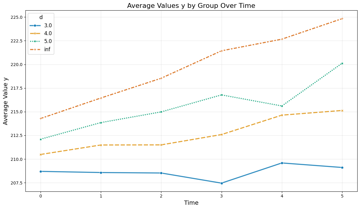
So let us take a look at the average values over time

[8]:

plot_data(agg_df, col_name='y')

/opt/hostedtoolcache/Python/3.12.11/x64/lib/python3.12/site-packages/matplotlib/colors.py:2295: RuntimeWarning: invalid value encountered in divide
  resdat /= (vmax - vmin)

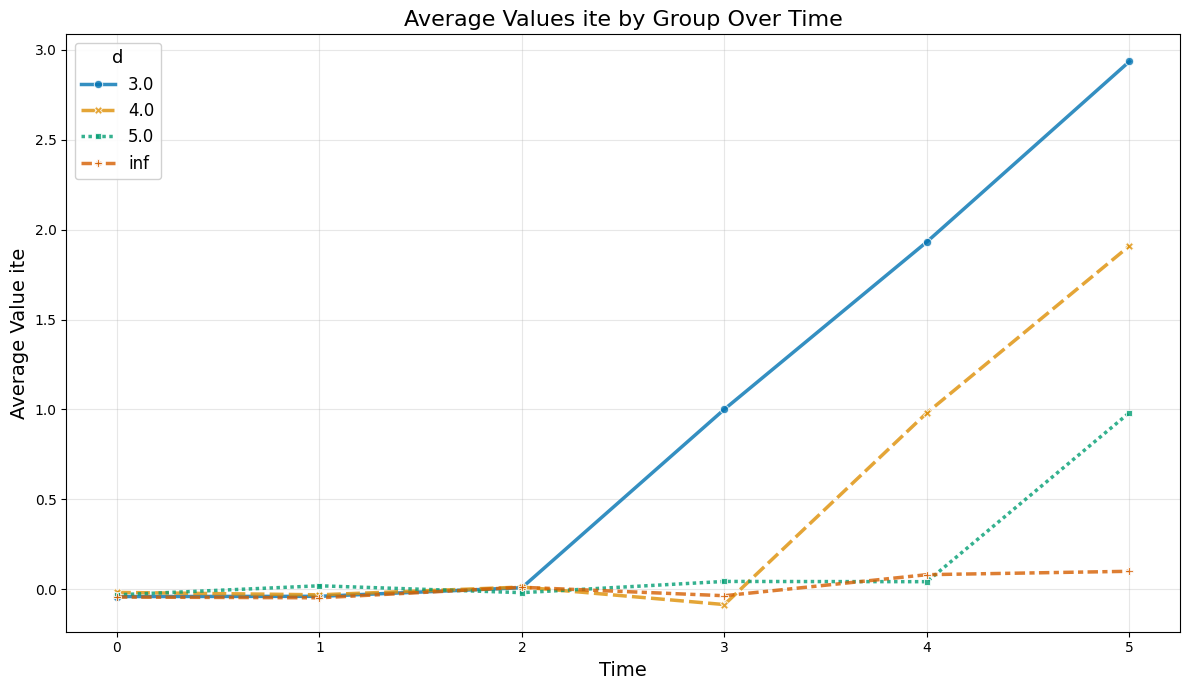
../../_images/examples_did_py_rep_cs_16_1.png

Instead the true average treatment treatment effects can be obtained by averaging (usually unobserved) the ite values.

The true effect just equals the exposure time (in months):

\[ATT(\mathrm{g}, t) = \min(\mathrm{t} - \mathrm{g} + 1, 0) =: e\]

[9]:

plot_data(agg_df, col_name='ite')

/opt/hostedtoolcache/Python/3.12.11/x64/lib/python3.12/site-packages/matplotlib/colors.py:2295: RuntimeWarning: invalid value encountered in divide
  resdat /= (vmax - vmin)

../../_images/examples_did_py_rep_cs_18_1.png

DoubleMLPanelData#

Finally, we can construct our DoubleMLPanelData, specifying

y_col : the outcome
d_cols: the group variable indicating the first treated period for each unit
id_col: the unique identification column for each unit
t_col : the time column
x_cols: the additional pre-treatment controls
datetime_unit: unit required for datetime columns and plotting

[10]:

dml_data = DoubleMLPanelData(
    data=df,
    y_col="y",
    d_cols="d",
    id_col="id",
    t_col="t",
    x_cols=["Z1", "Z2", "Z3", "Z4"],
)
print(dml_data)

================== DoubleMLPanelData Object ==================

------------------ Data summary      ------------------
Outcome variable: y
Treatment variable(s): ['d']
Covariates: ['Z1', 'Z2', 'Z3', 'Z4']
Instrument variable(s): None
Time variable: t
Id variable: id
No. Unique Ids: 9859
No. Observations: 29943

------------------ DataFrame info    ------------------
<class 'pandas.core.frame.DataFrame'>
RangeIndex: 29943 entries, 0 to 29942
Columns: 11 entries, id to ite
dtypes: float64(9), int64(2)
memory usage: 2.5 MB

ATT Estimation#

The DoubleML-package implements estimation of group-time average treatment effect via the DoubleMLDIDMulti class (see model documentation).

Basics#

The class basically behaves like other DoubleML classes and requires the specification of two learners (for more details on the regression elements, see score documentation).

The basic arguments of a DoubleMLDIDMulti object include

ml_g “outcome” regression learner
ml_m propensity Score learner
control_group the control group for the parallel trend assumption
gt_combinations combinations of \((\mathrm{g},t_\text{pre}, t_\text{eval})\)
anticipation_periods number of anticipation periods

We will construct a dict with “default” arguments.

For repeated cross-sectional data, we additionally specify the argument

panel=False

[11]:

default_args = {
    "ml_g": LGBMRegressor(n_estimators=500, learning_rate=0.01, verbose=-1, random_state=123),
    "ml_m": LGBMClassifier(n_estimators=500, learning_rate=0.01, verbose=-1, random_state=123),
    "control_group": "never_treated",
    "anticipation_periods": 0,
    "n_folds": 5,
    "n_rep": 1,
    "panel": False,
}

The model will be estimated using the fit() method.

[12]:

dml_obj = DoubleMLDIDMulti(dml_data, **default_args)
dml_obj.fit()
print(dml_obj)

================== DoubleMLDIDMulti Object ==================

------------------ Data summary      ------------------
Outcome variable: y
Treatment variable(s): ['d']
Covariates: ['Z1', 'Z2', 'Z3', 'Z4']
Instrument variable(s): None
Time variable: t
Id variable: id
No. Unique Ids: 9859
No. Observations: 29943

------------------ Score & algorithm ------------------
Score function: observational
Control group: never_treated
Anticipation periods: 0

------------------ Machine learner   ------------------
Learner ml_g: LGBMRegressor(learning_rate=0.01, n_estimators=500, random_state=123,
              verbose=-1)
Learner ml_m: LGBMClassifier(learning_rate=0.01, n_estimators=500, random_state=123,
               verbose=-1)
Out-of-sample Performance:
Regression:
Learner ml_g_d0_t0 RMSE: [[1.91322269 2.71397031 3.81480178 3.81741127 3.82812254 1.98813438
  2.75654332 3.85047387 5.26993438 5.15102386 1.97285903 2.7786232
  3.88584157 5.13073282 6.28539312]]
Learner ml_g_d0_t1 RMSE: [[2.80113584 3.86489394 5.32221113 6.31281923 7.39892758 2.71746733
  3.82316223 5.40216815 6.36422627 7.46228264 2.83033721 3.83280883
  5.14695833 6.25390044 7.44984806]]
Learner ml_g_d1_t0 RMSE: [[1.96737296 2.66307862 4.14649014 4.05695816 4.13584845 1.93231095
  2.93365857 4.03379093 5.19029113 5.04572511 1.96328786 2.96716842
  4.07103953 5.21151325 6.59834073]]
Learner ml_g_d1_t1 RMSE: [[2.63500518 4.14967599 4.97633864 5.62478948 7.30762583 2.92760366
  4.10373195 4.90172667 6.32556747 7.66390139 2.94223274 4.0512851
  5.19289748 6.53199139 7.37109331]]
Classification:
Learner ml_m Log Loss: [[0.60103305 0.60026782 0.5959583  0.59563249 0.59807237 0.62642966
  0.63249084 0.63229485 0.63140091 0.62462924 0.64636496 0.64892544
  0.6498445  0.64713937 0.64713091]]

------------------ Resampling        ------------------
No. folds: 5
No. repeated sample splits: 1

------------------ Fit summary       ------------------
                  coef   std err         t     P>|t|     2.5 %    97.5 %
ATT(3.0,0,1)  0.325001  0.265916  1.222193  0.221635 -0.196185  0.846186
ATT(3.0,1,2)  0.214740  0.284023  0.756064  0.449611 -0.341936  0.771415
ATT(3.0,2,3)  0.856617  0.416209  2.058142  0.039576  0.040863  1.672371
ATT(3.0,2,4)  1.657212  0.489385  3.386317  0.000708  0.698035  2.616389
ATT(3.0,2,5)  1.970993  0.495672  3.976406  0.000070  0.999494  2.942493
ATT(4.0,0,1)  0.194849  0.188758  1.032265  0.301948 -0.175111  0.564808
ATT(4.0,1,2) -0.006054  0.238342 -0.025400  0.979736 -0.473195  0.461087
ATT(4.0,2,3)  0.037167  0.314845  0.118048  0.906029 -0.579918  0.654252
ATT(4.0,3,4)  0.938008  0.438524  2.139011  0.032435  0.078516  1.797500
ATT(4.0,3,5)  2.214175  0.541790  4.086781  0.000044  1.152287  3.276063
ATT(5.0,0,1)  0.136159  0.159177  0.855395  0.392333 -0.175822  0.448140
ATT(5.0,1,2) -0.046409  0.214515 -0.216344  0.828719 -0.466850  0.374032
ATT(5.0,2,3) -0.273678  0.284639 -0.961494  0.336304 -0.831560  0.284203
ATT(5.0,3,4)  0.172444  0.398079  0.433190  0.664877 -0.607777  0.952665
ATT(5.0,4,5)  1.276653  0.500547  2.550518  0.010756  0.295600  2.257706

The summary displays estimates of the \(ATT(g,t_\text{eval})\) effects for different combinations of \((g,t_\text{eval})\) via \(\widehat{ATT}(\mathrm{g},t_\text{pre},t_\text{eval})\), where

\(\mathrm{g}\) specifies the group
\(t_\text{pre}\) specifies the corresponding pre-treatment period
\(t_\text{eval}\) specifies the evaluation period

The choice gt_combinations="standard", used estimates all possible combinations of \(ATT(g,t_\text{eval})\) via \(\widehat{ATT}(\mathrm{g},t_\text{pre},t_\text{eval})\), where the standard choice is \(t_\text{pre} = \min(\mathrm{g}, t_\text{eval}) - 1\) (without anticipation).

Remark that this includes pre-tests effects if \(\mathrm{g} > t_{eval}\), e.g. \(\widehat{ATT}(g=3, t_{\text{pre}}=0, t_{\text{eval}}=1)\) which estimates the pre-trend from time period \(0\) to \(1\) even if the actual treatment occured in time period \(3\).

As usual for the DoubleML-package, you can obtain joint confidence intervals via bootstrap.

[13]:

level = 0.95

ci = dml_obj.confint(level=level)
dml_obj.bootstrap(n_rep_boot=5000)
ci_joint = dml_obj.confint(level=level, joint=True)
ci_joint

[13]:

	2.5 %	97.5 %
ATT(3.0,0,1)	-0.448179	1.098181
ATT(3.0,1,2)	-0.611089	1.040569
ATT(3.0,2,3)	-0.353556	2.066789
ATT(3.0,2,4)	0.234272	3.080152
ATT(3.0,2,5)	0.529772	3.412214
ATT(4.0,0,1)	-0.353987	0.743685
ATT(4.0,1,2)	-0.699058	0.686951
ATT(4.0,2,3)	-0.878280	0.952614
ATT(4.0,3,4)	-0.337049	2.213066
ATT(4.0,3,5)	0.638862	3.789488
ATT(5.0,0,1)	-0.326665	0.598983
ATT(5.0,1,2)	-0.670134	0.577316
ATT(5.0,2,3)	-1.101297	0.553940
ATT(5.0,3,4)	-0.985015	1.329903
ATT(5.0,4,5)	-0.178741	2.732047

A visualization of the effects can be obtained via the plot_effects() method.

Remark that the plot used joint confidence intervals per default.

[14]:

dml_obj.plot_effects()

/opt/hostedtoolcache/Python/3.12.11/x64/lib/python3.12/site-packages/matplotlib/cbook.py:1719: FutureWarning: Calling float on a single element Series is deprecated and will raise a TypeError in the future. Use float(ser.iloc[0]) instead
  return math.isfinite(val)

[14]:

(<Figure size 1200x800 with 4 Axes>,
 [<Axes: title={'center': 'First Treated: 3.0'}, ylabel='Effect'>,
  <Axes: title={'center': 'First Treated: 4.0'}, ylabel='Effect'>,
  <Axes: title={'center': 'First Treated: 5.0'}, xlabel='Evaluation Period', ylabel='Effect'>])

../../_images/examples_did_py_rep_cs_30_2.png

Sensitivity Analysis#

As descripted in the Sensitivity Guide, robustness checks on omitted confounding/parallel trend violations are available, via the standard sensitivity_analysis() method.

[15]:

dml_obj.sensitivity_analysis()
print(dml_obj.sensitivity_summary)

================== Sensitivity Analysis ==================

------------------ Scenario          ------------------
Significance Level: level=0.95
Sensitivity parameters: cf_y=0.03; cf_d=0.03, rho=1.0

------------------ Bounds with CI    ------------------
              CI lower  theta lower     theta  theta upper  CI upper
ATT(3.0,0,1) -0.435002    -0.006549  0.325001     0.656550  1.109739
ATT(3.0,1,2) -0.749038    -0.273917  0.214740     0.703396  1.170138
ATT(3.0,2,3) -0.507803     0.204344  0.856617     1.508890  2.177685
ATT(3.0,2,4)  0.093256     0.918252  1.657212     2.396172  3.187992
ATT(3.0,2,5)  0.215082     1.034785  1.970993     2.907201  3.722757
ATT(4.0,0,1) -0.466102    -0.148451  0.194849     0.538148  0.842987
ATT(4.0,1,2) -0.891128    -0.494309 -0.006054     0.482202  0.871318
ATT(4.0,2,3) -1.123113    -0.604268  0.037167     0.678602  1.197898
ATT(4.0,3,4) -0.598886     0.127044  0.938008     1.748973  2.467963
ATT(4.0,3,5)  0.433387     1.325118  2.214175     3.103233  3.998013
ATT(5.0,0,1) -0.461116    -0.198254  0.136159     0.470572  0.732079
ATT(5.0,1,2) -0.865270    -0.510136 -0.046409     0.417318  0.768918
ATT(5.0,2,3) -1.366893    -0.897360 -0.273678     0.350003  0.818497
ATT(5.0,3,4) -1.264451    -0.608449  0.172444     0.953336  1.608720
ATT(5.0,4,5) -0.475183     0.350174  1.276653     2.203132  3.026724

------------------ Robustness Values ------------------
              H_0    RV (%)   RVa (%)
ATT(3.0,0,1)  0.0  2.941695  0.000638
ATT(3.0,1,2)  0.0  1.329777  0.000451
ATT(3.0,2,3)  0.0  3.921134  0.772547
ATT(3.0,2,4)  0.0  6.601803  3.360425
ATT(3.0,2,5)  0.0  6.210499  3.671291
ATT(4.0,0,1)  0.0  1.714089  0.000400
ATT(4.0,1,2)  0.0  0.037620  0.000445
ATT(4.0,2,3)  0.0  0.176193  0.000500
ATT(4.0,3,4)  0.0  3.461760  0.806811
ATT(4.0,3,5)  0.0  7.303806  4.423654
ATT(5.0,0,1)  0.0  1.232681  0.000649
ATT(5.0,1,2)  0.0  0.304222  0.000586
ATT(5.0,2,3)  0.0  1.327857  0.000403
ATT(5.0,3,4)  0.0  0.670553  0.000656
ATT(5.0,4,5)  0.0  4.110206  1.476942

In this example one can clearly, distinguish the robustness of the non-zero effects vs. the pre-treatment periods.

Control Groups#

The current implementation support the following control groups

"never_treated"
"not_yet_treated"

Remark that the ``”not_yet_treated” depends on anticipation.

For differences and recommendations, we refer to Callaway and Sant’Anna(2021).

[16]:

dml_obj_nyt = DoubleMLDIDMulti(dml_data, **(default_args | {"control_group": "not_yet_treated"}))
dml_obj_nyt.fit()
dml_obj_nyt.bootstrap(n_rep_boot=5000)
dml_obj_nyt.plot_effects()

/opt/hostedtoolcache/Python/3.12.11/x64/lib/python3.12/site-packages/matplotlib/cbook.py:1719: FutureWarning: Calling float on a single element Series is deprecated and will raise a TypeError in the future. Use float(ser.iloc[0]) instead
  return math.isfinite(val)

[16]:

(<Figure size 1200x800 with 4 Axes>,
 [<Axes: title={'center': 'First Treated: 3.0'}, ylabel='Effect'>,
  <Axes: title={'center': 'First Treated: 4.0'}, ylabel='Effect'>,
  <Axes: title={'center': 'First Treated: 5.0'}, xlabel='Evaluation Period', ylabel='Effect'>])

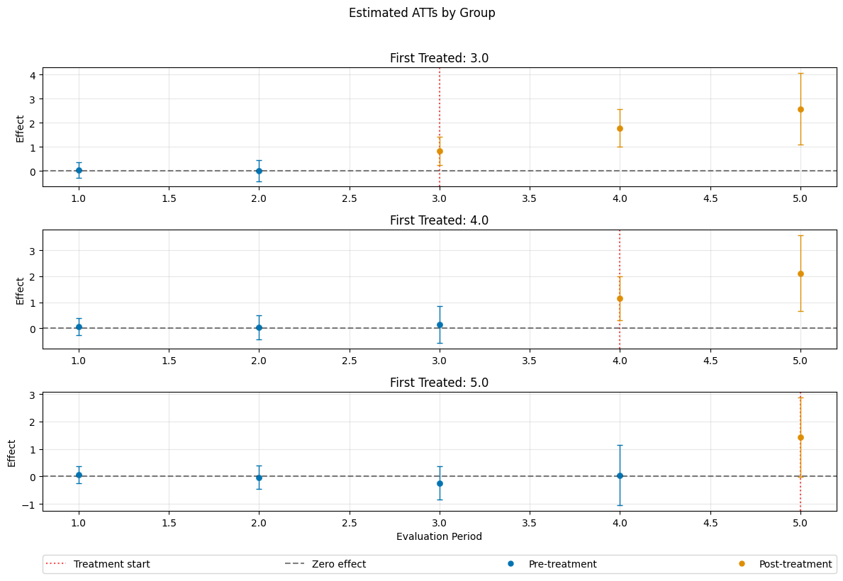
../../_images/examples_did_py_rep_cs_35_2.png

Linear Covariate Adjustment#

Remark that we relied on boosted trees to adjust for conditional parallel trends which allow for a nonlinear adjustment. In comparison to linear adjustment, we could rely on linear learners.

Remark that the DGP (``dgp_type=4``) is based on nonlinear conditional expectations such that the estimates will be biased

[17]:

linear_learners = {
    "ml_g": LinearRegression(),
    "ml_m": LogisticRegression(),
}

dml_obj_linear = DoubleMLDIDMulti(dml_data, **(default_args | linear_learners))
dml_obj_linear.fit()
dml_obj_linear.bootstrap(n_rep_boot=5000)
dml_obj_linear.plot_effects()

/opt/hostedtoolcache/Python/3.12.11/x64/lib/python3.12/site-packages/matplotlib/cbook.py:1719: FutureWarning: Calling float on a single element Series is deprecated and will raise a TypeError in the future. Use float(ser.iloc[0]) instead
  return math.isfinite(val)

[17]:

(<Figure size 1200x800 with 4 Axes>,
 [<Axes: title={'center': 'First Treated: 3.0'}, ylabel='Effect'>,
  <Axes: title={'center': 'First Treated: 4.0'}, ylabel='Effect'>,
  <Axes: title={'center': 'First Treated: 5.0'}, xlabel='Evaluation Period', ylabel='Effect'>])

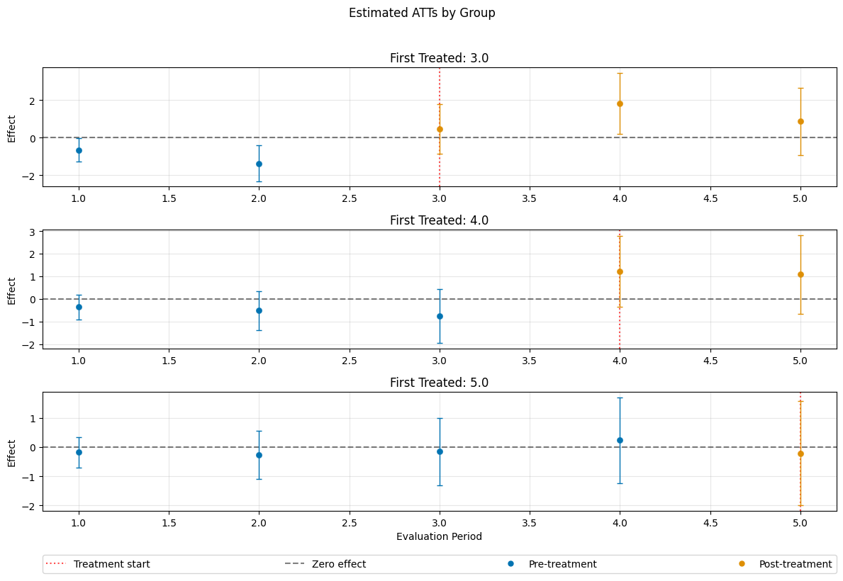
../../_images/examples_did_py_rep_cs_37_2.png

Aggregated Effects#

As the did-R-package, the \(ATT\)’s can be aggregated to summarize multiple effects. For details on different aggregations and details on their interpretations see Callaway and Sant’Anna(2021).

The aggregations are implemented via the aggregate() method.

Group Aggregation#

To obtain group-specific effects one can would like to average \(ATT(\mathrm{g}, t_\text{eval})\) over \(t_\text{eval}\). As a sample oracle we will combine all ite’s based on group \(\mathrm{g}\).

[18]:

df_post_treatment = df[df["t"] >= df["d"]]
df_post_treatment.groupby("d")["ite"].mean()

[18]:

d
3.0    1.970580
4.0    1.434381
5.0    0.981953
Name: ite, dtype: float64

To obtain group-specific effects it is possible to aggregate several \(\widehat{ATT}(\mathrm{g},t_\text{pre},t_\text{eval})\) values based on the group \(\mathrm{g}\) by setting the aggregation="group" argument.

[19]:

aggregated_group = dml_obj.aggregate(aggregation="group")
print(aggregated_group)
_ = aggregated_group.plot_effects()

================== DoubleMLDIDAggregation Object ==================
 Group Aggregation

------------------ Overall Aggregated Effects ------------------
    coef  std err        t        P>|t|    2.5 %   97.5 %
1.450825 0.237613 6.105843 1.022598e-09 0.985113 1.916537
------------------ Aggregated Effects         ------------------
         coef   std err         t     P>|t|     2.5 %    97.5 %
3.0  1.494941  0.308451  4.846612  0.000001  0.890388  2.099493
4.0  1.576092  0.383075  4.114316  0.000039  0.825279  2.326905
5.0  1.276653  0.500547  2.550518  0.010756  0.295600  2.257706
------------------ Additional Information     ------------------
Score function: observational
Control group: never_treated
Anticipation periods: 0

/home/runner/work/doubleml-docs/doubleml-docs/doubleml-for-py/doubleml/did/did_aggregation.py:368: UserWarning: Joint confidence intervals require bootstrapping which hasn't been performed yet. Automatically applying '.aggregated_frameworks.bootstrap(method="normal", n_rep_boot=500)' with default values. For different bootstrap settings, call bootstrap() explicitly before plotting.
  warnings.warn(

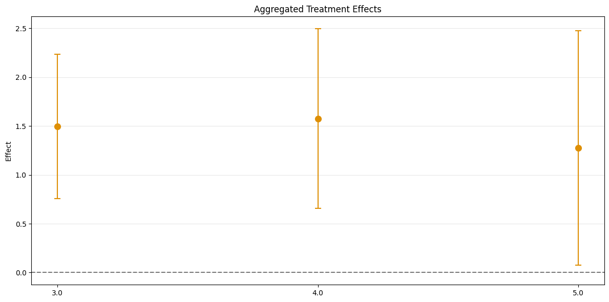
../../_images/examples_did_py_rep_cs_42_2.png

The output is a DoubleMLDIDAggregation object which includes an overall aggregation summary based on group size.

Time Aggregation#

To obtain time-specific effects one can would like to average \(ATT(\mathrm{g}, t_\text{eval})\) over \(\mathrm{g}\) (respecting group size). As a sample oracle we will combine all ite’s based on group \(\mathrm{g}\). As oracle values, we obtain

[20]:

df_post_treatment.groupby("t")["ite"].mean()

[20]:

t
3    1.000940
4    1.464804
5    1.967992
Name: ite, dtype: float64

To aggregate \(\widehat{ATT}(\mathrm{g},t_\text{pre},t_\text{eval})\), based on \(t_\text{eval}\), but weighted with respect to group size. Corresponds to Calendar Time Effects from the did-R-package.

For calendar time effects set aggregation="time".

[21]:

aggregated_time = dml_obj.aggregate("time")
print(aggregated_time)
fig, ax = aggregated_time.plot_effects()

================== DoubleMLDIDAggregation Object ==================
 Time Aggregation

------------------ Overall Aggregated Effects ------------------
    coef  std err        t        P>|t|    2.5 %   97.5 %
1.329206 0.216833 6.130086 8.783159e-10 0.904221 1.754191
------------------ Aggregated Effects         ------------------
       coef   std err         t     P>|t|     2.5 %    97.5 %
3  0.856617  0.416209  2.058142  0.039576  0.040863  1.672371
4  1.305270  0.379027  3.443737  0.000574  0.562390  2.048149
5  1.825730  0.382087  4.778315  0.000002  1.076854  2.574607
------------------ Additional Information     ------------------
Score function: observational
Control group: never_treated
Anticipation periods: 0

/home/runner/work/doubleml-docs/doubleml-docs/doubleml-for-py/doubleml/did/did_aggregation.py:368: UserWarning: Joint confidence intervals require bootstrapping which hasn't been performed yet. Automatically applying '.aggregated_frameworks.bootstrap(method="normal", n_rep_boot=500)' with default values. For different bootstrap settings, call bootstrap() explicitly before plotting.
  warnings.warn(

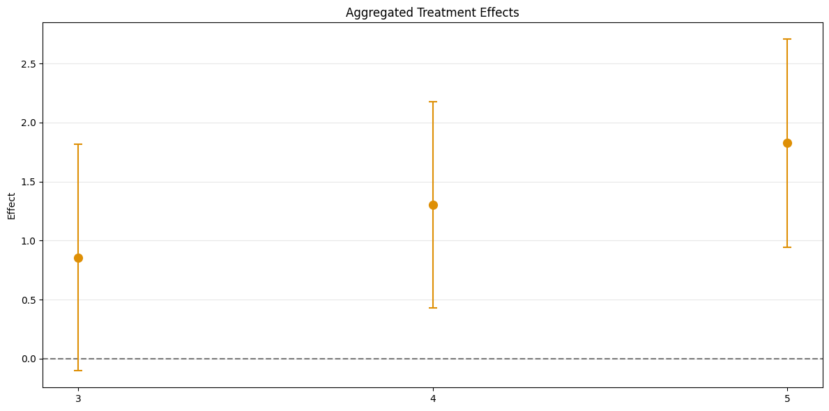
../../_images/examples_did_py_rep_cs_47_2.png

Event Study Aggregation#

To obtain event-study-type effects one can would like to aggregate \(ATT(\mathrm{g}, t_\text{eval})\) over \(e = t_\text{eval} - \mathrm{g}\) (respecting group size). As a sample oracle we will combine all ite’s based on group \(\mathrm{g}\). As oracle values, we obtain

[22]:

df_treated = df[df["d"] != np.inf].copy()
df_treated["e"] = df_treated["t"] - df_treated["d"]
df_treated.groupby("e")["ite"].mean().iloc[1:]

[22]:

e
-4.0    0.000054
-3.0   -0.030737
-2.0    0.003880
-1.0   -0.011715
 0.0    0.988017
 1.0    1.921556
 2.0    2.935983
Name: ite, dtype: float64

Analogously, aggregation="eventstudy" aggregates \(\widehat{ATT}(\mathrm{g},t_\text{pre},t_\text{eval})\) based on exposure time \(e = t_\text{eval} - \mathrm{g}\) (respecting group size).

[23]:

aggregated_eventstudy = dml_obj.aggregate("eventstudy")
print(aggregated_eventstudy)
aggregated_eventstudy.plot_effects()

================== DoubleMLDIDAggregation Object ==================
 Event Study Aggregation

------------------ Overall Aggregated Effects ------------------
    coef  std err        t        P>|t|    2.5 %   97.5 %
1.640245 0.273236 6.003035 1.936627e-09 1.104712 2.175778
------------------ Aggregated Effects         ------------------
          coef   std err         t         P>|t|     2.5 %    97.5 %
-4.0  0.136159  0.159177  0.855395  3.923328e-01 -0.175822  0.448140
-3.0  0.075222  0.126006  0.596973  5.505255e-01 -0.171744  0.322188
-2.0  0.021118  0.127518  0.165605  8.684681e-01 -0.228813  0.271048
-1.0  0.142335  0.164127  0.867229  3.858166e-01 -0.179347  0.464018
0.0   1.019979  0.208309  4.896473  9.757212e-07  0.611701  1.428258
1.0   1.929762  0.364340  5.296603  1.179767e-07  1.215670  2.643855
2.0   1.970993  0.495672  3.976406  6.996473e-05  0.999494  2.942493
------------------ Additional Information     ------------------
Score function: observational
Control group: never_treated
Anticipation periods: 0

/home/runner/work/doubleml-docs/doubleml-docs/doubleml-for-py/doubleml/did/did_aggregation.py:368: UserWarning: Joint confidence intervals require bootstrapping which hasn't been performed yet. Automatically applying '.aggregated_frameworks.bootstrap(method="normal", n_rep_boot=500)' with default values. For different bootstrap settings, call bootstrap() explicitly before plotting.
  warnings.warn(

[23]:

(<Figure size 1200x600 with 1 Axes>,
 <Axes: title={'center': 'Aggregated Treatment Effects'}, ylabel='Effect'>)

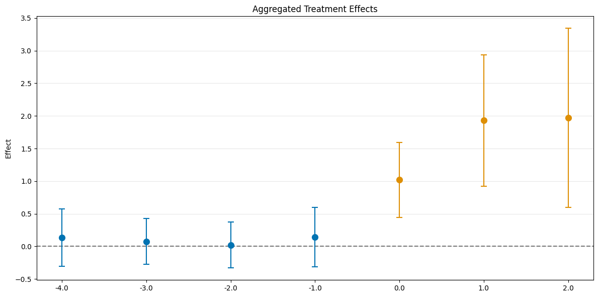
../../_images/examples_did_py_rep_cs_51_3.png

Aggregation Details#

The DoubleMLDIDAggregation objects include several DoubleMLFrameworks which support methods like bootstrap() or confint(). Further, the weights can be accessed via the properties

overall_aggregation_weights: weights for the overall aggregation
aggregation_weights: weights for the aggregation

To clarify, e.g. for the eventstudy aggregation

[24]:

print(aggregated_eventstudy)

================== DoubleMLDIDAggregation Object ==================
 Event Study Aggregation

------------------ Overall Aggregated Effects ------------------
    coef  std err        t        P>|t|    2.5 %   97.5 %
1.640245 0.273236 6.003035 1.936627e-09 1.104712 2.175778
------------------ Aggregated Effects         ------------------
          coef   std err         t         P>|t|     2.5 %    97.5 %
-4.0  0.136159  0.159177  0.855395  3.923328e-01 -0.175822  0.448140
-3.0  0.075222  0.126006  0.596973  5.505255e-01 -0.171744  0.322188
-2.0  0.021118  0.127518  0.165605  8.684681e-01 -0.228813  0.271048
-1.0  0.142335  0.164127  0.867229  3.858166e-01 -0.179347  0.464018
0.0   1.019979  0.208309  4.896473  9.757212e-07  0.611701  1.428258
1.0   1.929762  0.364340  5.296603  1.179767e-07  1.215670  2.643855
2.0   1.970993  0.495672  3.976406  6.996473e-05  0.999494  2.942493
------------------ Additional Information     ------------------
Score function: observational
Control group: never_treated
Anticipation periods: 0

Here, the overall effect aggregation aggregates each effect with positive exposure

[25]:

print(aggregated_eventstudy.overall_aggregation_weights)

[0.         0.         0.         0.         0.33333333 0.33333333
 0.33333333]

If one would like to consider how the aggregated effect with \(e=0\) is computed, one would have to look at the corresponding set of weights within the aggregation_weights property

[26]:

# the weights for e=0 correspond to the fifth element of the aggregation weights
aggregated_eventstudy.aggregation_weights[4]

[26]:

array([0.        , 0.        , 0.34473374, 0.        , 0.        ,
       0.        , 0.        , 0.        , 0.33035471, 0.        ,
       0.        , 0.        , 0.        , 0.        , 0.32491155])

Taking a look at the original dml_obj, one can see that this combines the following estimates (only show month):

\(\widehat{ATT}(04,03,04)\)
\(\widehat{ATT}(05,04,05)\)
\(\widehat{ATT}(06,05,06)\)

[27]:

print(dml_obj.summary["coef"])

ATT(3.0,0,1)    0.325001
ATT(3.0,1,2)    0.214740
ATT(3.0,2,3)    0.856617
ATT(3.0,2,4)    1.657212
ATT(3.0,2,5)    1.970993
ATT(4.0,0,1)    0.194849
ATT(4.0,1,2)   -0.006054
ATT(4.0,2,3)    0.037167
ATT(4.0,3,4)    0.938008
ATT(4.0,3,5)    2.214175
ATT(5.0,0,1)    0.136159
ATT(5.0,1,2)   -0.046409
ATT(5.0,2,3)   -0.273678
ATT(5.0,3,4)    0.172444
ATT(5.0,4,5)    1.276653
Name: coef, dtype: float64

Anticipation#

As described in the Model Guide, one can include anticipation periods \(\delta>0\) by setting the anticipation_periods parameter.

Data with Anticipation#

The DGP allows to include anticipation periods via the anticipation_periods parameter. In this case the observations will be “shifted” such that units anticipate the effect earlier and the exposure effect is increased by the number of periods where the effect is anticipated.

[28]:

n_obs = 4000
n_periods = 6

df_anticipation = make_did_cs_CS2021(n_obs, dgp_type=4, n_periods=n_periods, n_pre_treat_periods=3, time_type="datetime", anticipation_periods=1)

print(df_anticipation.shape)
df_anticipation.head()

(19213, 10)

[28]:

	id	y	y0	y1	d	t	Z1	Z2	Z3	Z4
1	0	199.655233	199.655233	196.683179	2025-04-01	2025-01-01	-1.189192	1.572002	-0.298420	0.230266
2	0	194.229213	194.229213	192.928194	2025-04-01	2025-02-01	-1.189192	1.572002	-0.298420	0.230266
4	0	185.050549	183.112574	185.050549	2025-04-01	2025-04-01	-1.189192	1.572002	-0.298420	0.230266
5	0	179.448724	178.642680	179.448724	2025-04-01	2025-05-01	-1.189192	1.572002	-0.298420	0.230266
9	1	210.898382	210.898382	213.009927	2025-04-01	2025-02-01	0.013028	0.243494	-0.068973	-0.701157

To visualize the anticipation, we will again plot the “oracle” values

[29]:

df_anticipation["ite"] = df_anticipation["y1"] - df_anticipation["y0"]
agg_df_anticipation = df_anticipation.groupby(["t", "d"]).agg(**agg_dictionary).reset_index()
agg_df_anticipation.head()

[29]:

	t	d	y_mean	y_lower_quantile	y_upper_quantile	ite_mean	ite_lower_quantile	ite_upper_quantile
0	2025-01-01	2025-04-01	208.273128	190.946129	224.787858	-0.044406	-2.226315	2.086865
1	2025-01-01	2025-05-01	211.136999	193.951770	227.753455	0.028734	-2.254275	2.235347
2	2025-01-01	2025-06-01	213.516989	196.512335	230.378492	-0.039991	-2.403552	2.357908
3	2025-02-01	2025-04-01	208.196777	183.101934	235.198722	-0.085253	-2.340793	2.126578
4	2025-02-01	2025-05-01	211.363358	186.764807	233.997283	-0.101928	-2.442010	2.279181

One can see that the effect is already anticipated one period before the actual treatment assignment.

[30]:

plot_data(agg_df_anticipation, col_name='ite')

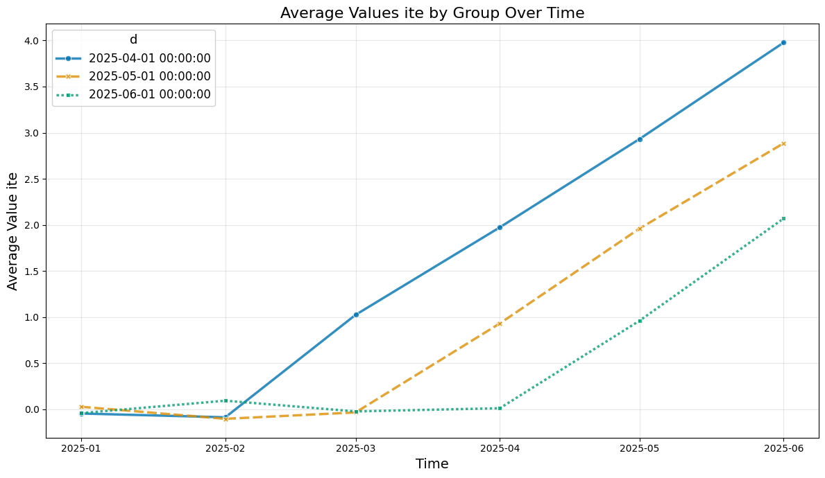
../../_images/examples_did_py_rep_cs_66_0.png

Initialize a corresponding DoubleMLPanelData object.

[31]:

dml_data_anticipation = DoubleMLPanelData(
    data=df_anticipation,
    y_col="y",
    d_cols="d",
    id_col="id",
    t_col="t",
    x_cols=["Z1", "Z2", "Z3", "Z4"],
    datetime_unit="M"
)

ATT Estimation#

Let us take a look at the estimation without anticipation.

[32]:

dml_obj_anticipation = DoubleMLDIDMulti(dml_data_anticipation, **default_args)
dml_obj_anticipation.fit()
dml_obj_anticipation.bootstrap(n_rep_boot=5000)
dml_obj_anticipation.plot_effects()

/opt/hostedtoolcache/Python/3.12.11/x64/lib/python3.12/site-packages/matplotlib/cbook.py:1719: FutureWarning: Calling float on a single element Series is deprecated and will raise a TypeError in the future. Use float(ser.iloc[0]) instead
  return math.isfinite(val)

[32]:

(<Figure size 1200x800 with 4 Axes>,
 [<Axes: title={'center': 'First Treated: 2025-04'}, ylabel='Effect'>,
  <Axes: title={'center': 'First Treated: 2025-05'}, ylabel='Effect'>,
  <Axes: title={'center': 'First Treated: 2025-06'}, xlabel='Evaluation Period', ylabel='Effect'>])

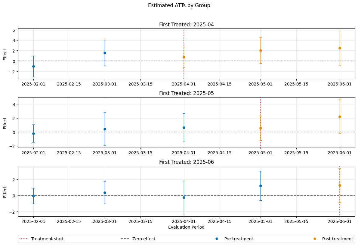
../../_images/examples_did_py_rep_cs_70_2.png

The effects are obviously biased. To include anticipation periods, one can adjust the anticipation_periods parameter. Correspondingly, the outcome regression (and not yet treated units) are adjusted.

[33]:

dml_obj_anticipation = DoubleMLDIDMulti(dml_data_anticipation, **(default_args| {"anticipation_periods": 1}))
dml_obj_anticipation.fit()
dml_obj_anticipation.bootstrap(n_rep_boot=5000)
dml_obj_anticipation.plot_effects()

/opt/hostedtoolcache/Python/3.12.11/x64/lib/python3.12/site-packages/matplotlib/cbook.py:1719: FutureWarning: Calling float on a single element Series is deprecated and will raise a TypeError in the future. Use float(ser.iloc[0]) instead
  return math.isfinite(val)
/opt/hostedtoolcache/Python/3.12.11/x64/lib/python3.12/site-packages/matplotlib/cbook.py:1719: FutureWarning: Calling float on a single element Series is deprecated and will raise a TypeError in the future. Use float(ser.iloc[0]) instead
  return math.isfinite(val)
/opt/hostedtoolcache/Python/3.12.11/x64/lib/python3.12/site-packages/matplotlib/cbook.py:1719: FutureWarning: Calling float on a single element Series is deprecated and will raise a TypeError in the future. Use float(ser.iloc[0]) instead
  return math.isfinite(val)
/opt/hostedtoolcache/Python/3.12.11/x64/lib/python3.12/site-packages/matplotlib/cbook.py:1719: FutureWarning: Calling float on a single element Series is deprecated and will raise a TypeError in the future. Use float(ser.iloc[0]) instead
  return math.isfinite(val)
/opt/hostedtoolcache/Python/3.12.11/x64/lib/python3.12/site-packages/matplotlib/cbook.py:1719: FutureWarning: Calling float on a single element Series is deprecated and will raise a TypeError in the future. Use float(ser.iloc[0]) instead
  return math.isfinite(val)

[33]:

(<Figure size 1200x800 with 4 Axes>,
 [<Axes: title={'center': 'First Treated: 2025-04'}, ylabel='Effect'>,
  <Axes: title={'center': 'First Treated: 2025-05'}, ylabel='Effect'>,
  <Axes: title={'center': 'First Treated: 2025-06'}, xlabel='Evaluation Period', ylabel='Effect'>])

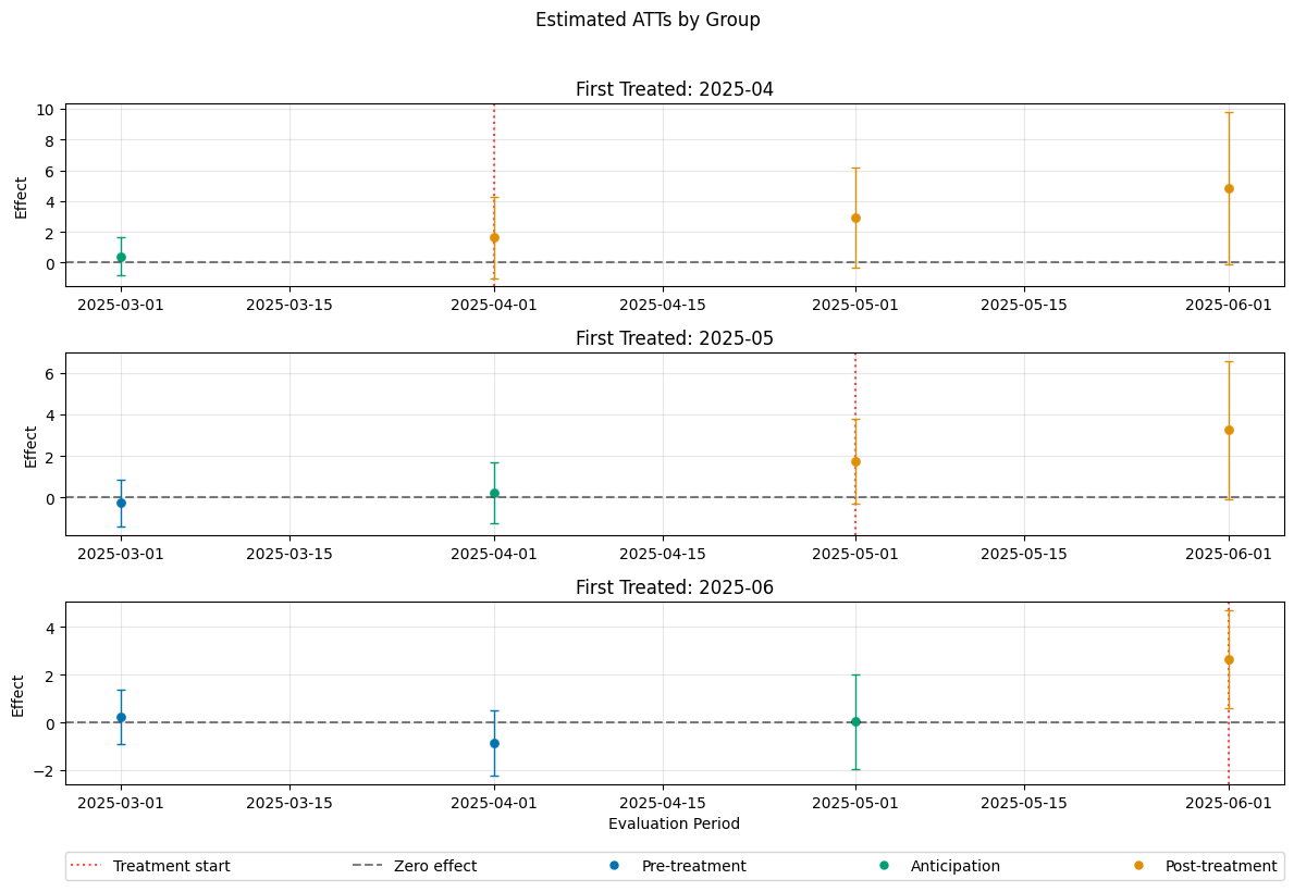
../../_images/examples_did_py_rep_cs_72_2.png

Group-Time Combinations#

The default option gt_combinations="standard" includes all group time values with the specific choice of \(t_\text{pre} = \min(\mathrm{g}, t_\text{eval}) - 1\) (without anticipation) which is the weakest possible parallel trend assumption.

Other options are possible or only specific combinations of \((\mathrm{g},t_\text{pre},t_\text{eval})\).

All combinations#

The option gt_combinations="all" includes all relevant group time values with \(t_\text{pre} < \min(\mathrm{g}, t_\text{eval})\), including longer parallel trend assumptions. This can result in multiple estimates for the same \(ATT(\mathrm{g},t)\), which have slightly different assumptions (length of parallel trends).

[34]:

dml_obj_all = DoubleMLDIDMulti(dml_data, **(default_args| {"gt_combinations": "all"}))
dml_obj_all.fit()
dml_obj_all.bootstrap(n_rep_boot=5000)
dml_obj_all.plot_effects()

[34]:

(<Figure size 1200x800 with 4 Axes>,
 [<Axes: title={'center': 'First Treated: 3.0'}, ylabel='Effect'>,
  <Axes: title={'center': 'First Treated: 4.0'}, ylabel='Effect'>,
  <Axes: title={'center': 'First Treated: 5.0'}, xlabel='Evaluation Period', ylabel='Effect'>])

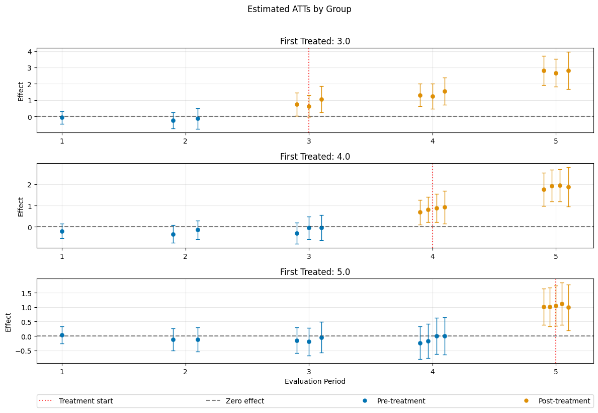
../../_images/examples_did_py_rep_cs_75_1.png

Universal Base Period#

The option gt_combinations="universal" set \(t_\text{pre} = \mathrm{g} - \delta - 1\), corresponding to a universal/constant comparison or base period.

Remark that this implies \(t_\text{pre} > t_\text{eval}\) for all pre-treatment periods (accounting for anticipation). Therefore these effects do not have the same straightforward interpretation as ATT’s.

[35]:

dml_obj_universal = DoubleMLDIDMulti(dml_data, **(default_args| {"gt_combinations": "universal"}))
dml_obj_universal.fit()
dml_obj_universal.bootstrap(n_rep_boot=5000)
dml_obj_universal.plot_effects()

/opt/hostedtoolcache/Python/3.12.11/x64/lib/python3.12/site-packages/matplotlib/cbook.py:1719: FutureWarning: Calling float on a single element Series is deprecated and will raise a TypeError in the future. Use float(ser.iloc[0]) instead
  return math.isfinite(val)

[35]:

(<Figure size 1200x800 with 4 Axes>,
 [<Axes: title={'center': 'First Treated: 3.0'}, ylabel='Effect'>,
  <Axes: title={'center': 'First Treated: 4.0'}, ylabel='Effect'>,
  <Axes: title={'center': 'First Treated: 5.0'}, xlabel='Evaluation Period', ylabel='Effect'>])

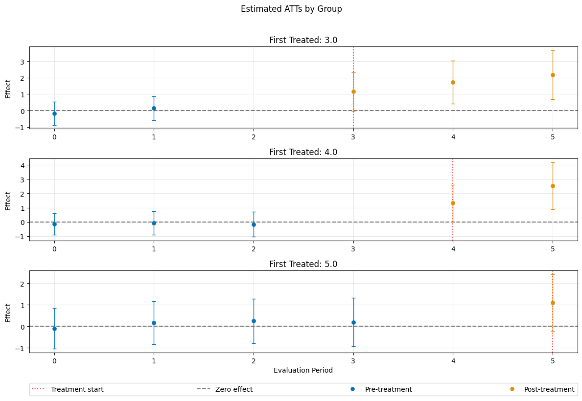
../../_images/examples_did_py_rep_cs_77_2.png

Selected Combinations#

Instead it is also possible to just submit a list of tuples containing \((\mathrm{g}, t_\text{pre}, t_\text{eval})\) combinations. E.g. only two combinations

[36]:

gt_dict = {
    "gt_combinations": [
        (4.0, 1, 2),
        (4.0, 1, 3),
        ]
}

dml_obj_all = DoubleMLDIDMulti(dml_data, **(default_args| gt_dict))
dml_obj_all.fit()
dml_obj_all.bootstrap(n_rep_boot=5000)
dml_obj_all.plot_effects()

[36]:

(<Figure size 1200x800 with 2 Axes>,
 [<Axes: title={'center': 'First Treated: 4.0'}, xlabel='Evaluation Period', ylabel='Effect'>])

../../_images/examples_did_py_rep_cs_79_1.png