Note
-
Download Jupyter notebook:
https://docs.doubleml.org/stable/examples/did/py_panel.ipynb.
Python: Panel Data with Multiple Time Periods#
In this example, a detailed guide on Difference-in-Differences with multiple time periods using the DoubleML-package. The implementation is based on Callaway and Sant’Anna(2021).
The notebook requires the following packages:
[1]:
import seaborn as sns
import matplotlib.pyplot as plt
import pandas as pd
import numpy as np

from lightgbm import LGBMRegressor, LGBMClassifier
from sklearn.linear_model import LinearRegression, LogisticRegression

from doubleml.did import DoubleMLDIDMulti
from doubleml.data import DoubleMLPanelData

from doubleml.did.datasets import make_did_CS2021
Data#
We will rely on the make_did_CS2021 DGP, which is inspired by Callaway and Sant’Anna(2021) (Appendix SC) and Sant’Anna and Zhao (2020).
We will observe n_obs units over n_periods. Remark that the dataframe includes observations of the potential outcomes y0 and y1, such that we can use oracle estimates as comparisons.
[2]:
n_obs = 5000
n_periods = 6

df = make_did_CS2021(n_obs, dgp_type=4, n_periods=n_periods, n_pre_treat_periods=3, time_type="datetime")
df["ite"] = df["y1"] - df["y0"]

print(df.shape)
df.head()
(30000, 11)
[2]:
| id | y | y0 | y1 | d | t | Z1 | Z2 | Z3 | Z4 | ite | |
|---|---|---|---|---|---|---|---|---|---|---|---|
| 0 | 0 | 214.648948 | 214.648948 | 216.526723 | NaT | 2025-01-01 | 0.814694 | -0.111789 | -0.714316 | -0.362425 | 1.877775 |
| 1 | 0 | 218.007494 | 218.007494 | 217.637084 | NaT | 2025-02-01 | 0.814694 | -0.111789 | -0.714316 | -0.362425 | -0.370410 |
| 2 | 0 | 220.876382 | 220.876382 | 220.593040 | NaT | 2025-03-01 | 0.814694 | -0.111789 | -0.714316 | -0.362425 | -0.283342 |
| 3 | 0 | 223.952998 | 223.952998 | 222.737394 | NaT | 2025-04-01 | 0.814694 | -0.111789 | -0.714316 | -0.362425 | -1.215604 |
| 4 | 0 | 225.864350 | 225.864350 | 227.075939 | NaT | 2025-05-01 | 0.814694 | -0.111789 | -0.714316 | -0.362425 | 1.211589 |
Data Details#
Here, we slightly abuse the definition of the potential outcomes. \(Y_{i,t}(1)\) corresponds to the (potential) outcome if unit \(i\) would have received treatment at time period \(\mathrm{g}\) (where the group \(\mathrm{g}\) is drawn with probabilities based on \(Z\)).
More specifically
where
\(f_t(Z)\) depends on pre-treatment observable covariates \(Z_1,\dots, Z_4\) and time \(t\)
\(\delta_t\) is a time fixed effect
\(\eta_i\) is a unit fixed effect
\(\epsilon_{i,t,\cdot}\) are time varying unobservables (iid. \(N(0,1)\))
\(\theta_{i,t,\mathrm{g}}\) correponds to the exposure effect of unit \(i\) based on group \(\mathrm{g}\) at time \(t\)
For the pre-treatment periods the exposure effect is set to
such that
The DoubleML Coverage Repository includes coverage simulations based on this DGP.
Data Description#
The data is a balanced panel where each unit is observed over n_periods starting Janary 2025.
[3]:
df.groupby("t").size()
[3]:
t
2025-01-01    5000
2025-02-01    5000
2025-03-01    5000
2025-04-01    5000
2025-05-01    5000
2025-06-01    5000
dtype: int64
The treatment column d indicates first treatment period of the corresponding unit, whereas NaT units are never treated.
Generally, never treated units should take either on the value ``np.inf`` or ``pd.NaT`` depending on the data type (``float`` or ``datetime``).
The individual units are roughly uniformly divided between the groups, where treatment assignment depends on the pre-treatment covariates Z1 to Z4.
[4]:
df.groupby("d", dropna=False).size()
[4]:
d
2025-04-01    7986
2025-05-01    6972
2025-06-01    7194
NaT           7848
dtype: int64
Here, the group indicates the first treated period and NaT units are never treated. To simplify plotting and pands
[5]:
df.groupby("d", dropna=False).size()
[5]:
d
2025-04-01    7986
2025-05-01    6972
2025-06-01    7194
NaT           7848
dtype: int64
To get a better understanding of the underlying data and true effects, we will compare the unconditional averages and the true effects based on the oracle values of individual effects ite.
[6]:
# rename for plotting
df["First Treated"] = df["d"].dt.strftime("%Y-%m").fillna("Never Treated")

# Create aggregation dictionary for means
def agg_dict(col_name):
    return {
        f'{col_name}_mean': (col_name, 'mean'),
        f'{col_name}_lower_quantile': (col_name, lambda x: x.quantile(0.05)),
        f'{col_name}_upper_quantile': (col_name, lambda x: x.quantile(0.95))
    }

# Calculate means and confidence intervals
agg_dictionary = agg_dict("y") | agg_dict("ite")

agg_df = df.groupby(["t", "First Treated"]).agg(**agg_dictionary).reset_index()
agg_df.head()
[6]:
| t | First Treated | y_mean | y_lower_quantile | y_upper_quantile | ite_mean | ite_lower_quantile | ite_upper_quantile | |
|---|---|---|---|---|---|---|---|---|
| 0 | 2025-01-01 | 2025-04 | 208.922460 | 198.590876 | 218.693719 | -0.013427 | -2.390291 | 2.397519 |
| 1 | 2025-01-01 | 2025-05 | 210.438795 | 200.311440 | 220.882262 | -0.049431 | -2.297203 | 2.228032 |
| 2 | 2025-01-01 | 2025-06 | 212.611488 | 202.480511 | 223.674050 | -0.022325 | -2.354440 | 2.378775 |
| 3 | 2025-01-01 | Never Treated | 214.219256 | 204.187176 | 224.204373 | 0.024217 | -2.319649 | 2.289477 |
| 4 | 2025-02-01 | 2025-04 | 208.781654 | 188.627032 | 227.042490 | 0.066124 | -2.292886 | 2.393307 |
[7]:
def plot_data(df, col_name='y'):
    """
    Create an improved plot with colorblind-friendly features

    Parameters:
    -----------
    df : DataFrame
        The dataframe containing the data
    col_name : str, default='y'
        Column name to plot (will use '{col_name}_mean')
    """
    plt.figure(figsize=(12, 7))
    n_colors = df["First Treated"].nunique()
    color_palette = sns.color_palette("colorblind", n_colors=n_colors)

    sns.lineplot(
        data=df,
        x='t',
        y=f'{col_name}_mean',
        hue='First Treated',
        style='First Treated',
        palette=color_palette,
        markers=True,
        dashes=True,
        linewidth=2.5,
        alpha=0.8
    )

    plt.title(f'Average Values {col_name} by Group Over Time', fontsize=16)
    plt.xlabel('Time', fontsize=14)
    plt.ylabel(f'Average Value {col_name}', fontsize=14)


    plt.legend(title='First Treated', title_fontsize=13, fontsize=12,
               frameon=True, framealpha=0.9, loc='best')

    plt.grid(alpha=0.3, linestyle='-')
    plt.tight_layout()

    plt.show()
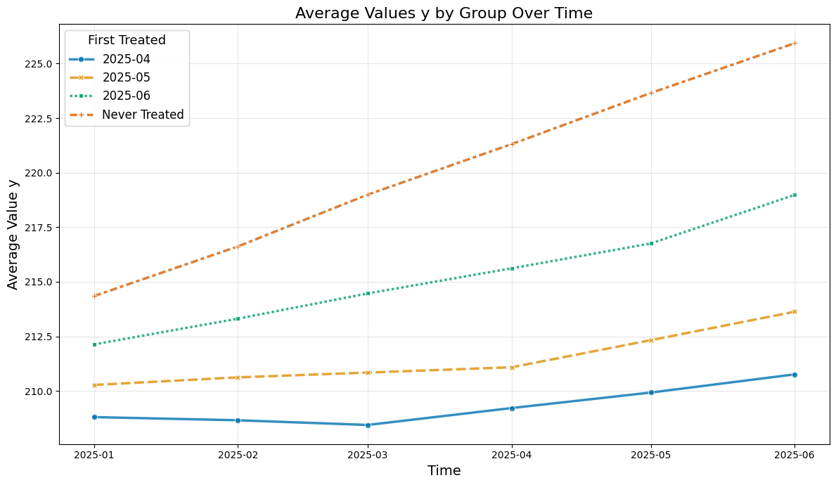
So let us take a look at the average values over time
[8]:
plot_data(agg_df, col_name='y')
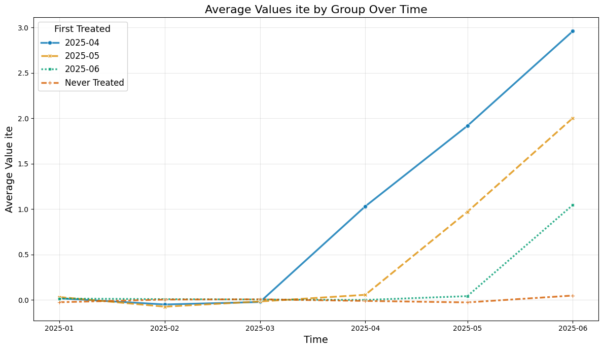
Instead the true average treatment treatment effects can be obtained by averaging (usually unobserved) the ite values.
The true effect just equals the exposure time (in months):
[9]:
plot_data(agg_df, col_name='ite')
DoubleMLPanelData#
Finally, we can construct our DoubleMLPanelData, specifying
y_col: the outcomed_cols: the group variable indicating the first treated period for each unitid_col: the unique identification column for each unitt_col: the time columnx_cols: the additional pre-treatment controlsdatetime_unit: unit required fordatetimecolumns and plotting
[10]:
dml_data = DoubleMLPanelData(
    data=df,
    y_col="y",
    d_cols="d",
    id_col="id",
    t_col="t",
    x_cols=["Z1", "Z2", "Z3", "Z4"],
    datetime_unit="M"
)
print(dml_data)
================== DoubleMLPanelData Object ==================

------------------ Data summary      ------------------
Outcome variable: y
Treatment variable(s): ['d']
Covariates: ['Z1', 'Z2', 'Z3', 'Z4']
Instrument variable(s): None
Time variable: t
Id variable: id
Static panel data: False
No. Unique Ids: 5000
No. Observations: 30000
------------------ DataFrame info    ------------------
<class 'pandas.DataFrame'>
RangeIndex: 30000 entries, 0 to 29999
Columns: 12 entries, id to First Treated
dtypes: datetime64[s](2), float64(8), int64(1), str(1)
memory usage: 2.7 MB
ATT Estimation#
The DoubleML-package implements estimation of group-time average treatment effect via the DoubleMLDIDMulti class (see model documentation).
Basics#
The class basically behaves like other DoubleML classes and requires the specification of two learners (for more details on the regression elements, see score documentation).
The basic arguments of a DoubleMLDIDMulti object include
ml_g“outcome” regression learnerml_mpropensity Score learnercontrol_groupthe control group for the parallel trend assumptiongt_combinationscombinations of \((\mathrm{g},t_\text{pre}, t_\text{eval})\)anticipation_periodsnumber of anticipation periods
We will construct a dict with “default” arguments.
[11]:
default_args = {
    "ml_g": LGBMRegressor(n_estimators=500, learning_rate=0.01, verbose=-1, random_state=123),
    "ml_m": LGBMClassifier(n_estimators=500, learning_rate=0.01, verbose=-1, random_state=123),
    "control_group": "never_treated",
    "gt_combinations": "standard",
    "anticipation_periods": 0,
    "n_folds": 5,
    "n_rep": 1,
}
The model will be estimated using the fit() method.
[12]:
np.random.seed(42)
dml_obj = DoubleMLDIDMulti(dml_data, **default_args)
dml_obj.fit()
print(dml_obj)
/opt/hostedtoolcache/Python/3.12.13/x64/lib/python3.12/site-packages/sklearn/utils/validation.py:2739: UserWarning: X does not have valid feature names, but LGBMRegressor was fitted with feature names
  warnings.warn(
/opt/hostedtoolcache/Python/3.12.13/x64/lib/python3.12/site-packages/sklearn/utils/validation.py:2739: UserWarning: X does not have valid feature names, but LGBMRegressor was fitted with feature names
  warnings.warn(
/opt/hostedtoolcache/Python/3.12.13/x64/lib/python3.12/site-packages/sklearn/utils/validation.py:2739: UserWarning: X does not have valid feature names, but LGBMRegressor was fitted with feature names
  warnings.warn(
/opt/hostedtoolcache/Python/3.12.13/x64/lib/python3.12/site-packages/sklearn/utils/validation.py:2739: UserWarning: X does not have valid feature names, but LGBMRegressor was fitted with feature names
  warnings.warn(
/opt/hostedtoolcache/Python/3.12.13/x64/lib/python3.12/site-packages/sklearn/utils/validation.py:2739: UserWarning: X does not have valid feature names, but LGBMRegressor was fitted with feature names
  warnings.warn(
/opt/hostedtoolcache/Python/3.12.13/x64/lib/python3.12/site-packages/sklearn/utils/validation.py:2739: UserWarning: X does not have valid feature names, but LGBMRegressor was fitted with feature names
  warnings.warn(
/opt/hostedtoolcache/Python/3.12.13/x64/lib/python3.12/site-packages/sklearn/utils/validation.py:2739: UserWarning: X does not have valid feature names, but LGBMRegressor was fitted with feature names
  warnings.warn(
/opt/hostedtoolcache/Python/3.12.13/x64/lib/python3.12/site-packages/sklearn/utils/validation.py:2739: UserWarning: X does not have valid feature names, but LGBMRegressor was fitted with feature names
  warnings.warn(
/opt/hostedtoolcache/Python/3.12.13/x64/lib/python3.12/site-packages/sklearn/utils/validation.py:2739: UserWarning: X does not have valid feature names, but LGBMRegressor was fitted with feature names
  warnings.warn(
/opt/hostedtoolcache/Python/3.12.13/x64/lib/python3.12/site-packages/sklearn/utils/validation.py:2739: UserWarning: X does not have valid feature names, but LGBMRegressor was fitted with feature names
  warnings.warn(
/opt/hostedtoolcache/Python/3.12.13/x64/lib/python3.12/site-packages/sklearn/utils/validation.py:2739: UserWarning: X does not have valid feature names, but LGBMClassifier was fitted with feature names
  warnings.warn(
/opt/hostedtoolcache/Python/3.12.13/x64/lib/python3.12/site-packages/sklearn/utils/validation.py:2739: UserWarning: X does not have valid feature names, but LGBMClassifier was fitted with feature names
  warnings.warn(
/opt/hostedtoolcache/Python/3.12.13/x64/lib/python3.12/site-packages/sklearn/utils/validation.py:2739: UserWarning: X does not have valid feature names, but LGBMClassifier was fitted with feature names
  warnings.warn(
/opt/hostedtoolcache/Python/3.12.13/x64/lib/python3.12/site-packages/sklearn/utils/validation.py:2739: UserWarning: X does not have valid feature names, but LGBMClassifier was fitted with feature names
  warnings.warn(
/opt/hostedtoolcache/Python/3.12.13/x64/lib/python3.12/site-packages/sklearn/utils/validation.py:2739: UserWarning: X does not have valid feature names, but LGBMClassifier was fitted with feature names
  warnings.warn(
/opt/hostedtoolcache/Python/3.12.13/x64/lib/python3.12/site-packages/sklearn/utils/validation.py:2739: UserWarning: X does not have valid feature names, but LGBMRegressor was fitted with feature names
  warnings.warn(
/opt/hostedtoolcache/Python/3.12.13/x64/lib/python3.12/site-packages/sklearn/utils/validation.py:2739: UserWarning: X does not have valid feature names, but LGBMRegressor was fitted with feature names
  warnings.warn(
/opt/hostedtoolcache/Python/3.12.13/x64/lib/python3.12/site-packages/sklearn/utils/validation.py:2739: UserWarning: X does not have valid feature names, but LGBMRegressor was fitted with feature names
  warnings.warn(
/opt/hostedtoolcache/Python/3.12.13/x64/lib/python3.12/site-packages/sklearn/utils/validation.py:2739: UserWarning: X does not have valid feature names, but LGBMRegressor was fitted with feature names
  warnings.warn(
/opt/hostedtoolcache/Python/3.12.13/x64/lib/python3.12/site-packages/sklearn/utils/validation.py:2739: UserWarning: X does not have valid feature names, but LGBMRegressor was fitted with feature names
  warnings.warn(
/opt/hostedtoolcache/Python/3.12.13/x64/lib/python3.12/site-packages/sklearn/utils/validation.py:2739: UserWarning: X does not have valid feature names, but LGBMRegressor was fitted with feature names
  warnings.warn(
/opt/hostedtoolcache/Python/3.12.13/x64/lib/python3.12/site-packages/sklearn/utils/validation.py:2739: UserWarning: X does not have valid feature names, but LGBMRegressor was fitted with feature names
  warnings.warn(
/opt/hostedtoolcache/Python/3.12.13/x64/lib/python3.12/site-packages/sklearn/utils/validation.py:2739: UserWarning: X does not have valid feature names, but LGBMRegressor was fitted with feature names
  warnings.warn(
/opt/hostedtoolcache/Python/3.12.13/x64/lib/python3.12/site-packages/sklearn/utils/validation.py:2739: UserWarning: X does not have valid feature names, but LGBMRegressor was fitted with feature names
  warnings.warn(
/opt/hostedtoolcache/Python/3.12.13/x64/lib/python3.12/site-packages/sklearn/utils/validation.py:2739: UserWarning: X does not have valid feature names, but LGBMRegressor was fitted with feature names
  warnings.warn(
/opt/hostedtoolcache/Python/3.12.13/x64/lib/python3.12/site-packages/sklearn/utils/validation.py:2739: UserWarning: X does not have valid feature names, but LGBMClassifier was fitted with feature names
  warnings.warn(
/opt/hostedtoolcache/Python/3.12.13/x64/lib/python3.12/site-packages/sklearn/utils/validation.py:2739: UserWarning: X does not have valid feature names, but LGBMClassifier was fitted with feature names
  warnings.warn(
/opt/hostedtoolcache/Python/3.12.13/x64/lib/python3.12/site-packages/sklearn/utils/validation.py:2739: UserWarning: X does not have valid feature names, but LGBMClassifier was fitted with feature names
  warnings.warn(
/opt/hostedtoolcache/Python/3.12.13/x64/lib/python3.12/site-packages/sklearn/utils/validation.py:2739: UserWarning: X does not have valid feature names, but LGBMClassifier was fitted with feature names
  warnings.warn(
/opt/hostedtoolcache/Python/3.12.13/x64/lib/python3.12/site-packages/sklearn/utils/validation.py:2739: UserWarning: X does not have valid feature names, but LGBMClassifier was fitted with feature names
  warnings.warn(
/opt/hostedtoolcache/Python/3.12.13/x64/lib/python3.12/site-packages/sklearn/utils/validation.py:2739: UserWarning: X does not have valid feature names, but LGBMRegressor was fitted with feature names
  warnings.warn(
/opt/hostedtoolcache/Python/3.12.13/x64/lib/python3.12/site-packages/sklearn/utils/validation.py:2739: UserWarning: X does not have valid feature names, but LGBMRegressor was fitted with feature names
  warnings.warn(
/opt/hostedtoolcache/Python/3.12.13/x64/lib/python3.12/site-packages/sklearn/utils/validation.py:2739: UserWarning: X does not have valid feature names, but LGBMRegressor was fitted with feature names
  warnings.warn(
/opt/hostedtoolcache/Python/3.12.13/x64/lib/python3.12/site-packages/sklearn/utils/validation.py:2739: UserWarning: X does not have valid feature names, but LGBMRegressor was fitted with feature names
  warnings.warn(
/opt/hostedtoolcache/Python/3.12.13/x64/lib/python3.12/site-packages/sklearn/utils/validation.py:2739: UserWarning: X does not have valid feature names, but LGBMRegressor was fitted with feature names
  warnings.warn(
/opt/hostedtoolcache/Python/3.12.13/x64/lib/python3.12/site-packages/sklearn/utils/validation.py:2739: UserWarning: X does not have valid feature names, but LGBMRegressor was fitted with feature names
  warnings.warn(
/opt/hostedtoolcache/Python/3.12.13/x64/lib/python3.12/site-packages/sklearn/utils/validation.py:2739: UserWarning: X does not have valid feature names, but LGBMRegressor was fitted with feature names
  warnings.warn(
/opt/hostedtoolcache/Python/3.12.13/x64/lib/python3.12/site-packages/sklearn/utils/validation.py:2739: UserWarning: X does not have valid feature names, but LGBMRegressor was fitted with feature names
  warnings.warn(
/opt/hostedtoolcache/Python/3.12.13/x64/lib/python3.12/site-packages/sklearn/utils/validation.py:2739: UserWarning: X does not have valid feature names, but LGBMRegressor was fitted with feature names
  warnings.warn(
/opt/hostedtoolcache/Python/3.12.13/x64/lib/python3.12/site-packages/sklearn/utils/validation.py:2739: UserWarning: X does not have valid feature names, but LGBMRegressor was fitted with feature names
  warnings.warn(
/opt/hostedtoolcache/Python/3.12.13/x64/lib/python3.12/site-packages/sklearn/utils/validation.py:2739: UserWarning: X does not have valid feature names, but LGBMClassifier was fitted with feature names
  warnings.warn(
/opt/hostedtoolcache/Python/3.12.13/x64/lib/python3.12/site-packages/sklearn/utils/validation.py:2739: UserWarning: X does not have valid feature names, but LGBMClassifier was fitted with feature names
  warnings.warn(
/opt/hostedtoolcache/Python/3.12.13/x64/lib/python3.12/site-packages/sklearn/utils/validation.py:2739: UserWarning: X does not have valid feature names, but LGBMClassifier was fitted with feature names
  warnings.warn(
/opt/hostedtoolcache/Python/3.12.13/x64/lib/python3.12/site-packages/sklearn/utils/validation.py:2739: UserWarning: X does not have valid feature names, but LGBMClassifier was fitted with feature names
  warnings.warn(
/opt/hostedtoolcache/Python/3.12.13/x64/lib/python3.12/site-packages/sklearn/utils/validation.py:2739: UserWarning: X does not have valid feature names, but LGBMClassifier was fitted with feature names
  warnings.warn(
/opt/hostedtoolcache/Python/3.12.13/x64/lib/python3.12/site-packages/sklearn/utils/validation.py:2739: UserWarning: X does not have valid feature names, but LGBMRegressor was fitted with feature names
  warnings.warn(
/opt/hostedtoolcache/Python/3.12.13/x64/lib/python3.12/site-packages/sklearn/utils/validation.py:2739: UserWarning: X does not have valid feature names, but LGBMRegressor was fitted with feature names
  warnings.warn(
/opt/hostedtoolcache/Python/3.12.13/x64/lib/python3.12/site-packages/sklearn/utils/validation.py:2739: UserWarning: X does not have valid feature names, but LGBMRegressor was fitted with feature names
  warnings.warn(
/opt/hostedtoolcache/Python/3.12.13/x64/lib/python3.12/site-packages/sklearn/utils/validation.py:2739: UserWarning: X does not have valid feature names, but LGBMRegressor was fitted with feature names
  warnings.warn(
/opt/hostedtoolcache/Python/3.12.13/x64/lib/python3.12/site-packages/sklearn/utils/validation.py:2739: UserWarning: X does not have valid feature names, but LGBMRegressor was fitted with feature names
  warnings.warn(
/opt/hostedtoolcache/Python/3.12.13/x64/lib/python3.12/site-packages/sklearn/utils/validation.py:2739: UserWarning: X does not have valid feature names, but LGBMRegressor was fitted with feature names
  warnings.warn(
/opt/hostedtoolcache/Python/3.12.13/x64/lib/python3.12/site-packages/sklearn/utils/validation.py:2739: UserWarning: X does not have valid feature names, but LGBMRegressor was fitted with feature names
  warnings.warn(
/opt/hostedtoolcache/Python/3.12.13/x64/lib/python3.12/site-packages/sklearn/utils/validation.py:2739: UserWarning: X does not have valid feature names, but LGBMRegressor was fitted with feature names
  warnings.warn(
/opt/hostedtoolcache/Python/3.12.13/x64/lib/python3.12/site-packages/sklearn/utils/validation.py:2739: UserWarning: X does not have valid feature names, but LGBMRegressor was fitted with feature names
  warnings.warn(
/opt/hostedtoolcache/Python/3.12.13/x64/lib/python3.12/site-packages/sklearn/utils/validation.py:2739: UserWarning: X does not have valid feature names, but LGBMRegressor was fitted with feature names
  warnings.warn(
/opt/hostedtoolcache/Python/3.12.13/x64/lib/python3.12/site-packages/sklearn/utils/validation.py:2739: UserWarning: X does not have valid feature names, but LGBMClassifier was fitted with feature names
  warnings.warn(
/opt/hostedtoolcache/Python/3.12.13/x64/lib/python3.12/site-packages/sklearn/utils/validation.py:2739: UserWarning: X does not have valid feature names, but LGBMClassifier was fitted with feature names
  warnings.warn(
/opt/hostedtoolcache/Python/3.12.13/x64/lib/python3.12/site-packages/sklearn/utils/validation.py:2739: UserWarning: X does not have valid feature names, but LGBMClassifier was fitted with feature names
  warnings.warn(
/opt/hostedtoolcache/Python/3.12.13/x64/lib/python3.12/site-packages/sklearn/utils/validation.py:2739: UserWarning: X does not have valid feature names, but LGBMClassifier was fitted with feature names
  warnings.warn(
/opt/hostedtoolcache/Python/3.12.13/x64/lib/python3.12/site-packages/sklearn/utils/validation.py:2739: UserWarning: X does not have valid feature names, but LGBMClassifier was fitted with feature names
  warnings.warn(
/opt/hostedtoolcache/Python/3.12.13/x64/lib/python3.12/site-packages/sklearn/utils/validation.py:2739: UserWarning: X does not have valid feature names, but LGBMRegressor was fitted with feature names
  warnings.warn(
/opt/hostedtoolcache/Python/3.12.13/x64/lib/python3.12/site-packages/sklearn/utils/validation.py:2739: UserWarning: X does not have valid feature names, but LGBMRegressor was fitted with feature names
  warnings.warn(
/opt/hostedtoolcache/Python/3.12.13/x64/lib/python3.12/site-packages/sklearn/utils/validation.py:2739: UserWarning: X does not have valid feature names, but LGBMRegressor was fitted with feature names
  warnings.warn(
/opt/hostedtoolcache/Python/3.12.13/x64/lib/python3.12/site-packages/sklearn/utils/validation.py:2739: UserWarning: X does not have valid feature names, but LGBMRegressor was fitted with feature names
  warnings.warn(
/opt/hostedtoolcache/Python/3.12.13/x64/lib/python3.12/site-packages/sklearn/utils/validation.py:2739: UserWarning: X does not have valid feature names, but LGBMRegressor was fitted with feature names
  warnings.warn(
/opt/hostedtoolcache/Python/3.12.13/x64/lib/python3.12/site-packages/sklearn/utils/validation.py:2739: UserWarning: X does not have valid feature names, but LGBMRegressor was fitted with feature names
  warnings.warn(
/opt/hostedtoolcache/Python/3.12.13/x64/lib/python3.12/site-packages/sklearn/utils/validation.py:2739: UserWarning: X does not have valid feature names, but LGBMRegressor was fitted with feature names
  warnings.warn(
/opt/hostedtoolcache/Python/3.12.13/x64/lib/python3.12/site-packages/sklearn/utils/validation.py:2739: UserWarning: X does not have valid feature names, but LGBMRegressor was fitted with feature names
  warnings.warn(
/opt/hostedtoolcache/Python/3.12.13/x64/lib/python3.12/site-packages/sklearn/utils/validation.py:2739: UserWarning: X does not have valid feature names, but LGBMRegressor was fitted with feature names
  warnings.warn(
/opt/hostedtoolcache/Python/3.12.13/x64/lib/python3.12/site-packages/sklearn/utils/validation.py:2739: UserWarning: X does not have valid feature names, but LGBMRegressor was fitted with feature names
  warnings.warn(
/opt/hostedtoolcache/Python/3.12.13/x64/lib/python3.12/site-packages/sklearn/utils/validation.py:2739: UserWarning: X does not have valid feature names, but LGBMClassifier was fitted with feature names
  warnings.warn(
/opt/hostedtoolcache/Python/3.12.13/x64/lib/python3.12/site-packages/sklearn/utils/validation.py:2739: UserWarning: X does not have valid feature names, but LGBMClassifier was fitted with feature names
  warnings.warn(
/opt/hostedtoolcache/Python/3.12.13/x64/lib/python3.12/site-packages/sklearn/utils/validation.py:2739: UserWarning: X does not have valid feature names, but LGBMClassifier was fitted with feature names
  warnings.warn(
/opt/hostedtoolcache/Python/3.12.13/x64/lib/python3.12/site-packages/sklearn/utils/validation.py:2739: UserWarning: X does not have valid feature names, but LGBMClassifier was fitted with feature names
  warnings.warn(
/opt/hostedtoolcache/Python/3.12.13/x64/lib/python3.12/site-packages/sklearn/utils/validation.py:2739: UserWarning: X does not have valid feature names, but LGBMClassifier was fitted with feature names
  warnings.warn(
/opt/hostedtoolcache/Python/3.12.13/x64/lib/python3.12/site-packages/sklearn/utils/validation.py:2739: UserWarning: X does not have valid feature names, but LGBMRegressor was fitted with feature names
  warnings.warn(
/opt/hostedtoolcache/Python/3.12.13/x64/lib/python3.12/site-packages/sklearn/utils/validation.py:2739: UserWarning: X does not have valid feature names, but LGBMRegressor was fitted with feature names
  warnings.warn(
/opt/hostedtoolcache/Python/3.12.13/x64/lib/python3.12/site-packages/sklearn/utils/validation.py:2739: UserWarning: X does not have valid feature names, but LGBMRegressor was fitted with feature names
  warnings.warn(
/opt/hostedtoolcache/Python/3.12.13/x64/lib/python3.12/site-packages/sklearn/utils/validation.py:2739: UserWarning: X does not have valid feature names, but LGBMRegressor was fitted with feature names
  warnings.warn(
/opt/hostedtoolcache/Python/3.12.13/x64/lib/python3.12/site-packages/sklearn/utils/validation.py:2739: UserWarning: X does not have valid feature names, but LGBMRegressor was fitted with feature names
  warnings.warn(
/opt/hostedtoolcache/Python/3.12.13/x64/lib/python3.12/site-packages/sklearn/utils/validation.py:2739: UserWarning: X does not have valid feature names, but LGBMRegressor was fitted with feature names
  warnings.warn(
/opt/hostedtoolcache/Python/3.12.13/x64/lib/python3.12/site-packages/sklearn/utils/validation.py:2739: UserWarning: X does not have valid feature names, but LGBMRegressor was fitted with feature names
  warnings.warn(
/opt/hostedtoolcache/Python/3.12.13/x64/lib/python3.12/site-packages/sklearn/utils/validation.py:2739: UserWarning: X does not have valid feature names, but LGBMRegressor was fitted with feature names
  warnings.warn(
/opt/hostedtoolcache/Python/3.12.13/x64/lib/python3.12/site-packages/sklearn/utils/validation.py:2739: UserWarning: X does not have valid feature names, but LGBMRegressor was fitted with feature names
  warnings.warn(
/opt/hostedtoolcache/Python/3.12.13/x64/lib/python3.12/site-packages/sklearn/utils/validation.py:2739: UserWarning: X does not have valid feature names, but LGBMRegressor was fitted with feature names
  warnings.warn(
/opt/hostedtoolcache/Python/3.12.13/x64/lib/python3.12/site-packages/sklearn/utils/validation.py:2739: UserWarning: X does not have valid feature names, but LGBMClassifier was fitted with feature names
  warnings.warn(
/opt/hostedtoolcache/Python/3.12.13/x64/lib/python3.12/site-packages/sklearn/utils/validation.py:2739: UserWarning: X does not have valid feature names, but LGBMClassifier was fitted with feature names
  warnings.warn(
/opt/hostedtoolcache/Python/3.12.13/x64/lib/python3.12/site-packages/sklearn/utils/validation.py:2739: UserWarning: X does not have valid feature names, but LGBMClassifier was fitted with feature names
  warnings.warn(
/opt/hostedtoolcache/Python/3.12.13/x64/lib/python3.12/site-packages/sklearn/utils/validation.py:2739: UserWarning: X does not have valid feature names, but LGBMClassifier was fitted with feature names
  warnings.warn(
/opt/hostedtoolcache/Python/3.12.13/x64/lib/python3.12/site-packages/sklearn/utils/validation.py:2739: UserWarning: X does not have valid feature names, but LGBMClassifier was fitted with feature names
  warnings.warn(
/opt/hostedtoolcache/Python/3.12.13/x64/lib/python3.12/site-packages/sklearn/utils/validation.py:2739: UserWarning: X does not have valid feature names, but LGBMRegressor was fitted with feature names
  warnings.warn(
/opt/hostedtoolcache/Python/3.12.13/x64/lib/python3.12/site-packages/sklearn/utils/validation.py:2739: UserWarning: X does not have valid feature names, but LGBMRegressor was fitted with feature names
  warnings.warn(
/opt/hostedtoolcache/Python/3.12.13/x64/lib/python3.12/site-packages/sklearn/utils/validation.py:2739: UserWarning: X does not have valid feature names, but LGBMRegressor was fitted with feature names
  warnings.warn(
/opt/hostedtoolcache/Python/3.12.13/x64/lib/python3.12/site-packages/sklearn/utils/validation.py:2739: UserWarning: X does not have valid feature names, but LGBMRegressor was fitted with feature names
  warnings.warn(
/opt/hostedtoolcache/Python/3.12.13/x64/lib/python3.12/site-packages/sklearn/utils/validation.py:2739: UserWarning: X does not have valid feature names, but LGBMRegressor was fitted with feature names
  warnings.warn(
/opt/hostedtoolcache/Python/3.12.13/x64/lib/python3.12/site-packages/sklearn/utils/validation.py:2739: UserWarning: X does not have valid feature names, but LGBMRegressor was fitted with feature names
  warnings.warn(
/opt/hostedtoolcache/Python/3.12.13/x64/lib/python3.12/site-packages/sklearn/utils/validation.py:2739: UserWarning: X does not have valid feature names, but LGBMRegressor was fitted with feature names
  warnings.warn(
/opt/hostedtoolcache/Python/3.12.13/x64/lib/python3.12/site-packages/sklearn/utils/validation.py:2739: UserWarning: X does not have valid feature names, but LGBMRegressor was fitted with feature names
  warnings.warn(
/opt/hostedtoolcache/Python/3.12.13/x64/lib/python3.12/site-packages/sklearn/utils/validation.py:2739: UserWarning: X does not have valid feature names, but LGBMRegressor was fitted with feature names
  warnings.warn(
/opt/hostedtoolcache/Python/3.12.13/x64/lib/python3.12/site-packages/sklearn/utils/validation.py:2739: UserWarning: X does not have valid feature names, but LGBMRegressor was fitted with feature names
  warnings.warn(
/opt/hostedtoolcache/Python/3.12.13/x64/lib/python3.12/site-packages/sklearn/utils/validation.py:2739: UserWarning: X does not have valid feature names, but LGBMClassifier was fitted with feature names
  warnings.warn(
/opt/hostedtoolcache/Python/3.12.13/x64/lib/python3.12/site-packages/sklearn/utils/validation.py:2739: UserWarning: X does not have valid feature names, but LGBMClassifier was fitted with feature names
  warnings.warn(
/opt/hostedtoolcache/Python/3.12.13/x64/lib/python3.12/site-packages/sklearn/utils/validation.py:2739: UserWarning: X does not have valid feature names, but LGBMClassifier was fitted with feature names
  warnings.warn(
/opt/hostedtoolcache/Python/3.12.13/x64/lib/python3.12/site-packages/sklearn/utils/validation.py:2739: UserWarning: X does not have valid feature names, but LGBMClassifier was fitted with feature names
  warnings.warn(
/opt/hostedtoolcache/Python/3.12.13/x64/lib/python3.12/site-packages/sklearn/utils/validation.py:2739: UserWarning: X does not have valid feature names, but LGBMClassifier was fitted with feature names
  warnings.warn(
/opt/hostedtoolcache/Python/3.12.13/x64/lib/python3.12/site-packages/sklearn/utils/validation.py:2739: UserWarning: X does not have valid feature names, but LGBMRegressor was fitted with feature names
  warnings.warn(
/opt/hostedtoolcache/Python/3.12.13/x64/lib/python3.12/site-packages/sklearn/utils/validation.py:2739: UserWarning: X does not have valid feature names, but LGBMRegressor was fitted with feature names
  warnings.warn(
/opt/hostedtoolcache/Python/3.12.13/x64/lib/python3.12/site-packages/sklearn/utils/validation.py:2739: UserWarning: X does not have valid feature names, but LGBMRegressor was fitted with feature names
  warnings.warn(
/opt/hostedtoolcache/Python/3.12.13/x64/lib/python3.12/site-packages/sklearn/utils/validation.py:2739: UserWarning: X does not have valid feature names, but LGBMRegressor was fitted with feature names
  warnings.warn(
/opt/hostedtoolcache/Python/3.12.13/x64/lib/python3.12/site-packages/sklearn/utils/validation.py:2739: UserWarning: X does not have valid feature names, but LGBMRegressor was fitted with feature names
  warnings.warn(
/opt/hostedtoolcache/Python/3.12.13/x64/lib/python3.12/site-packages/sklearn/utils/validation.py:2739: UserWarning: X does not have valid feature names, but LGBMRegressor was fitted with feature names
  warnings.warn(
/opt/hostedtoolcache/Python/3.12.13/x64/lib/python3.12/site-packages/sklearn/utils/validation.py:2739: UserWarning: X does not have valid feature names, but LGBMRegressor was fitted with feature names
  warnings.warn(
/opt/hostedtoolcache/Python/3.12.13/x64/lib/python3.12/site-packages/sklearn/utils/validation.py:2739: UserWarning: X does not have valid feature names, but LGBMRegressor was fitted with feature names
  warnings.warn(
/opt/hostedtoolcache/Python/3.12.13/x64/lib/python3.12/site-packages/sklearn/utils/validation.py:2739: UserWarning: X does not have valid feature names, but LGBMRegressor was fitted with feature names
  warnings.warn(
/opt/hostedtoolcache/Python/3.12.13/x64/lib/python3.12/site-packages/sklearn/utils/validation.py:2739: UserWarning: X does not have valid feature names, but LGBMRegressor was fitted with feature names
  warnings.warn(
/opt/hostedtoolcache/Python/3.12.13/x64/lib/python3.12/site-packages/sklearn/utils/validation.py:2739: UserWarning: X does not have valid feature names, but LGBMClassifier was fitted with feature names
  warnings.warn(
/opt/hostedtoolcache/Python/3.12.13/x64/lib/python3.12/site-packages/sklearn/utils/validation.py:2739: UserWarning: X does not have valid feature names, but LGBMClassifier was fitted with feature names
  warnings.warn(
/opt/hostedtoolcache/Python/3.12.13/x64/lib/python3.12/site-packages/sklearn/utils/validation.py:2739: UserWarning: X does not have valid feature names, but LGBMClassifier was fitted with feature names
  warnings.warn(
/opt/hostedtoolcache/Python/3.12.13/x64/lib/python3.12/site-packages/sklearn/utils/validation.py:2739: UserWarning: X does not have valid feature names, but LGBMClassifier was fitted with feature names
  warnings.warn(
/opt/hostedtoolcache/Python/3.12.13/x64/lib/python3.12/site-packages/sklearn/utils/validation.py:2739: UserWarning: X does not have valid feature names, but LGBMClassifier was fitted with feature names
  warnings.warn(
/opt/hostedtoolcache/Python/3.12.13/x64/lib/python3.12/site-packages/sklearn/utils/validation.py:2739: UserWarning: X does not have valid feature names, but LGBMRegressor was fitted with feature names
  warnings.warn(
/opt/hostedtoolcache/Python/3.12.13/x64/lib/python3.12/site-packages/sklearn/utils/validation.py:2739: UserWarning: X does not have valid feature names, but LGBMRegressor was fitted with feature names
  warnings.warn(
/opt/hostedtoolcache/Python/3.12.13/x64/lib/python3.12/site-packages/sklearn/utils/validation.py:2739: UserWarning: X does not have valid feature names, but LGBMRegressor was fitted with feature names
  warnings.warn(
/opt/hostedtoolcache/Python/3.12.13/x64/lib/python3.12/site-packages/sklearn/utils/validation.py:2739: UserWarning: X does not have valid feature names, but LGBMRegressor was fitted with feature names
  warnings.warn(
/opt/hostedtoolcache/Python/3.12.13/x64/lib/python3.12/site-packages/sklearn/utils/validation.py:2739: UserWarning: X does not have valid feature names, but LGBMRegressor was fitted with feature names
  warnings.warn(
/opt/hostedtoolcache/Python/3.12.13/x64/lib/python3.12/site-packages/sklearn/utils/validation.py:2739: UserWarning: X does not have valid feature names, but LGBMRegressor was fitted with feature names
  warnings.warn(
/opt/hostedtoolcache/Python/3.12.13/x64/lib/python3.12/site-packages/sklearn/utils/validation.py:2739: UserWarning: X does not have valid feature names, but LGBMRegressor was fitted with feature names
  warnings.warn(
/opt/hostedtoolcache/Python/3.12.13/x64/lib/python3.12/site-packages/sklearn/utils/validation.py:2739: UserWarning: X does not have valid feature names, but LGBMRegressor was fitted with feature names
  warnings.warn(
/opt/hostedtoolcache/Python/3.12.13/x64/lib/python3.12/site-packages/sklearn/utils/validation.py:2739: UserWarning: X does not have valid feature names, but LGBMRegressor was fitted with feature names
  warnings.warn(
/opt/hostedtoolcache/Python/3.12.13/x64/lib/python3.12/site-packages/sklearn/utils/validation.py:2739: UserWarning: X does not have valid feature names, but LGBMRegressor was fitted with feature names
  warnings.warn(
/opt/hostedtoolcache/Python/3.12.13/x64/lib/python3.12/site-packages/sklearn/utils/validation.py:2739: UserWarning: X does not have valid feature names, but LGBMClassifier was fitted with feature names
  warnings.warn(
/opt/hostedtoolcache/Python/3.12.13/x64/lib/python3.12/site-packages/sklearn/utils/validation.py:2739: UserWarning: X does not have valid feature names, but LGBMClassifier was fitted with feature names
  warnings.warn(
/opt/hostedtoolcache/Python/3.12.13/x64/lib/python3.12/site-packages/sklearn/utils/validation.py:2739: UserWarning: X does not have valid feature names, but LGBMClassifier was fitted with feature names
  warnings.warn(
/opt/hostedtoolcache/Python/3.12.13/x64/lib/python3.12/site-packages/sklearn/utils/validation.py:2739: UserWarning: X does not have valid feature names, but LGBMClassifier was fitted with feature names
  warnings.warn(
/opt/hostedtoolcache/Python/3.12.13/x64/lib/python3.12/site-packages/sklearn/utils/validation.py:2739: UserWarning: X does not have valid feature names, but LGBMClassifier was fitted with feature names
  warnings.warn(
/opt/hostedtoolcache/Python/3.12.13/x64/lib/python3.12/site-packages/sklearn/utils/validation.py:2739: UserWarning: X does not have valid feature names, but LGBMRegressor was fitted with feature names
  warnings.warn(
/opt/hostedtoolcache/Python/3.12.13/x64/lib/python3.12/site-packages/sklearn/utils/validation.py:2739: UserWarning: X does not have valid feature names, but LGBMRegressor was fitted with feature names
  warnings.warn(
/opt/hostedtoolcache/Python/3.12.13/x64/lib/python3.12/site-packages/sklearn/utils/validation.py:2739: UserWarning: X does not have valid feature names, but LGBMRegressor was fitted with feature names
  warnings.warn(
/opt/hostedtoolcache/Python/3.12.13/x64/lib/python3.12/site-packages/sklearn/utils/validation.py:2739: UserWarning: X does not have valid feature names, but LGBMRegressor was fitted with feature names
  warnings.warn(
/opt/hostedtoolcache/Python/3.12.13/x64/lib/python3.12/site-packages/sklearn/utils/validation.py:2739: UserWarning: X does not have valid feature names, but LGBMRegressor was fitted with feature names
  warnings.warn(
/opt/hostedtoolcache/Python/3.12.13/x64/lib/python3.12/site-packages/sklearn/utils/validation.py:2739: UserWarning: X does not have valid feature names, but LGBMRegressor was fitted with feature names
  warnings.warn(
/opt/hostedtoolcache/Python/3.12.13/x64/lib/python3.12/site-packages/sklearn/utils/validation.py:2739: UserWarning: X does not have valid feature names, but LGBMRegressor was fitted with feature names
  warnings.warn(
/opt/hostedtoolcache/Python/3.12.13/x64/lib/python3.12/site-packages/sklearn/utils/validation.py:2739: UserWarning: X does not have valid feature names, but LGBMRegressor was fitted with feature names
  warnings.warn(
/opt/hostedtoolcache/Python/3.12.13/x64/lib/python3.12/site-packages/sklearn/utils/validation.py:2739: UserWarning: X does not have valid feature names, but LGBMRegressor was fitted with feature names
  warnings.warn(
/opt/hostedtoolcache/Python/3.12.13/x64/lib/python3.12/site-packages/sklearn/utils/validation.py:2739: UserWarning: X does not have valid feature names, but LGBMRegressor was fitted with feature names
  warnings.warn(
/opt/hostedtoolcache/Python/3.12.13/x64/lib/python3.12/site-packages/sklearn/utils/validation.py:2739: UserWarning: X does not have valid feature names, but LGBMClassifier was fitted with feature names
  warnings.warn(
/opt/hostedtoolcache/Python/3.12.13/x64/lib/python3.12/site-packages/sklearn/utils/validation.py:2739: UserWarning: X does not have valid feature names, but LGBMClassifier was fitted with feature names
  warnings.warn(
/opt/hostedtoolcache/Python/3.12.13/x64/lib/python3.12/site-packages/sklearn/utils/validation.py:2739: UserWarning: X does not have valid feature names, but LGBMClassifier was fitted with feature names
  warnings.warn(
/opt/hostedtoolcache/Python/3.12.13/x64/lib/python3.12/site-packages/sklearn/utils/validation.py:2739: UserWarning: X does not have valid feature names, but LGBMClassifier was fitted with feature names
  warnings.warn(
/opt/hostedtoolcache/Python/3.12.13/x64/lib/python3.12/site-packages/sklearn/utils/validation.py:2739: UserWarning: X does not have valid feature names, but LGBMClassifier was fitted with feature names
  warnings.warn(
/opt/hostedtoolcache/Python/3.12.13/x64/lib/python3.12/site-packages/sklearn/utils/validation.py:2739: UserWarning: X does not have valid feature names, but LGBMRegressor was fitted with feature names
  warnings.warn(
/opt/hostedtoolcache/Python/3.12.13/x64/lib/python3.12/site-packages/sklearn/utils/validation.py:2739: UserWarning: X does not have valid feature names, but LGBMRegressor was fitted with feature names
  warnings.warn(
/opt/hostedtoolcache/Python/3.12.13/x64/lib/python3.12/site-packages/sklearn/utils/validation.py:2739: UserWarning: X does not have valid feature names, but LGBMRegressor was fitted with feature names
  warnings.warn(
/opt/hostedtoolcache/Python/3.12.13/x64/lib/python3.12/site-packages/sklearn/utils/validation.py:2739: UserWarning: X does not have valid feature names, but LGBMRegressor was fitted with feature names
  warnings.warn(
/opt/hostedtoolcache/Python/3.12.13/x64/lib/python3.12/site-packages/sklearn/utils/validation.py:2739: UserWarning: X does not have valid feature names, but LGBMRegressor was fitted with feature names
  warnings.warn(
/opt/hostedtoolcache/Python/3.12.13/x64/lib/python3.12/site-packages/sklearn/utils/validation.py:2739: UserWarning: X does not have valid feature names, but LGBMRegressor was fitted with feature names
  warnings.warn(
/opt/hostedtoolcache/Python/3.12.13/x64/lib/python3.12/site-packages/sklearn/utils/validation.py:2739: UserWarning: X does not have valid feature names, but LGBMRegressor was fitted with feature names
  warnings.warn(
/opt/hostedtoolcache/Python/3.12.13/x64/lib/python3.12/site-packages/sklearn/utils/validation.py:2739: UserWarning: X does not have valid feature names, but LGBMRegressor was fitted with feature names
  warnings.warn(
/opt/hostedtoolcache/Python/3.12.13/x64/lib/python3.12/site-packages/sklearn/utils/validation.py:2739: UserWarning: X does not have valid feature names, but LGBMRegressor was fitted with feature names
  warnings.warn(
/opt/hostedtoolcache/Python/3.12.13/x64/lib/python3.12/site-packages/sklearn/utils/validation.py:2739: UserWarning: X does not have valid feature names, but LGBMRegressor was fitted with feature names
  warnings.warn(
/opt/hostedtoolcache/Python/3.12.13/x64/lib/python3.12/site-packages/sklearn/utils/validation.py:2739: UserWarning: X does not have valid feature names, but LGBMClassifier was fitted with feature names
  warnings.warn(
/opt/hostedtoolcache/Python/3.12.13/x64/lib/python3.12/site-packages/sklearn/utils/validation.py:2739: UserWarning: X does not have valid feature names, but LGBMClassifier was fitted with feature names
  warnings.warn(
/opt/hostedtoolcache/Python/3.12.13/x64/lib/python3.12/site-packages/sklearn/utils/validation.py:2739: UserWarning: X does not have valid feature names, but LGBMClassifier was fitted with feature names
  warnings.warn(
/opt/hostedtoolcache/Python/3.12.13/x64/lib/python3.12/site-packages/sklearn/utils/validation.py:2739: UserWarning: X does not have valid feature names, but LGBMClassifier was fitted with feature names
  warnings.warn(
/opt/hostedtoolcache/Python/3.12.13/x64/lib/python3.12/site-packages/sklearn/utils/validation.py:2739: UserWarning: X does not have valid feature names, but LGBMClassifier was fitted with feature names
  warnings.warn(
/opt/hostedtoolcache/Python/3.12.13/x64/lib/python3.12/site-packages/sklearn/utils/validation.py:2739: UserWarning: X does not have valid feature names, but LGBMRegressor was fitted with feature names
  warnings.warn(
/opt/hostedtoolcache/Python/3.12.13/x64/lib/python3.12/site-packages/sklearn/utils/validation.py:2739: UserWarning: X does not have valid feature names, but LGBMRegressor was fitted with feature names
  warnings.warn(
/opt/hostedtoolcache/Python/3.12.13/x64/lib/python3.12/site-packages/sklearn/utils/validation.py:2739: UserWarning: X does not have valid feature names, but LGBMRegressor was fitted with feature names
  warnings.warn(
/opt/hostedtoolcache/Python/3.12.13/x64/lib/python3.12/site-packages/sklearn/utils/validation.py:2739: UserWarning: X does not have valid feature names, but LGBMRegressor was fitted with feature names
  warnings.warn(
/opt/hostedtoolcache/Python/3.12.13/x64/lib/python3.12/site-packages/sklearn/utils/validation.py:2739: UserWarning: X does not have valid feature names, but LGBMRegressor was fitted with feature names
  warnings.warn(
/opt/hostedtoolcache/Python/3.12.13/x64/lib/python3.12/site-packages/sklearn/utils/validation.py:2739: UserWarning: X does not have valid feature names, but LGBMRegressor was fitted with feature names
  warnings.warn(
/opt/hostedtoolcache/Python/3.12.13/x64/lib/python3.12/site-packages/sklearn/utils/validation.py:2739: UserWarning: X does not have valid feature names, but LGBMRegressor was fitted with feature names
  warnings.warn(
/opt/hostedtoolcache/Python/3.12.13/x64/lib/python3.12/site-packages/sklearn/utils/validation.py:2739: UserWarning: X does not have valid feature names, but LGBMRegressor was fitted with feature names
  warnings.warn(
/opt/hostedtoolcache/Python/3.12.13/x64/lib/python3.12/site-packages/sklearn/utils/validation.py:2739: UserWarning: X does not have valid feature names, but LGBMRegressor was fitted with feature names
  warnings.warn(
/opt/hostedtoolcache/Python/3.12.13/x64/lib/python3.12/site-packages/sklearn/utils/validation.py:2739: UserWarning: X does not have valid feature names, but LGBMRegressor was fitted with feature names
  warnings.warn(
/opt/hostedtoolcache/Python/3.12.13/x64/lib/python3.12/site-packages/sklearn/utils/validation.py:2739: UserWarning: X does not have valid feature names, but LGBMClassifier was fitted with feature names
  warnings.warn(
/opt/hostedtoolcache/Python/3.12.13/x64/lib/python3.12/site-packages/sklearn/utils/validation.py:2739: UserWarning: X does not have valid feature names, but LGBMClassifier was fitted with feature names
  warnings.warn(
/opt/hostedtoolcache/Python/3.12.13/x64/lib/python3.12/site-packages/sklearn/utils/validation.py:2739: UserWarning: X does not have valid feature names, but LGBMClassifier was fitted with feature names
  warnings.warn(
/opt/hostedtoolcache/Python/3.12.13/x64/lib/python3.12/site-packages/sklearn/utils/validation.py:2739: UserWarning: X does not have valid feature names, but LGBMClassifier was fitted with feature names
  warnings.warn(
/opt/hostedtoolcache/Python/3.12.13/x64/lib/python3.12/site-packages/sklearn/utils/validation.py:2739: UserWarning: X does not have valid feature names, but LGBMClassifier was fitted with feature names
  warnings.warn(
/opt/hostedtoolcache/Python/3.12.13/x64/lib/python3.12/site-packages/sklearn/utils/validation.py:2739: UserWarning: X does not have valid feature names, but LGBMRegressor was fitted with feature names
  warnings.warn(
/opt/hostedtoolcache/Python/3.12.13/x64/lib/python3.12/site-packages/sklearn/utils/validation.py:2739: UserWarning: X does not have valid feature names, but LGBMRegressor was fitted with feature names
  warnings.warn(
/opt/hostedtoolcache/Python/3.12.13/x64/lib/python3.12/site-packages/sklearn/utils/validation.py:2739: UserWarning: X does not have valid feature names, but LGBMRegressor was fitted with feature names
  warnings.warn(
/opt/hostedtoolcache/Python/3.12.13/x64/lib/python3.12/site-packages/sklearn/utils/validation.py:2739: UserWarning: X does not have valid feature names, but LGBMRegressor was fitted with feature names
  warnings.warn(
/opt/hostedtoolcache/Python/3.12.13/x64/lib/python3.12/site-packages/sklearn/utils/validation.py:2739: UserWarning: X does not have valid feature names, but LGBMRegressor was fitted with feature names
  warnings.warn(
/opt/hostedtoolcache/Python/3.12.13/x64/lib/python3.12/site-packages/sklearn/utils/validation.py:2739: UserWarning: X does not have valid feature names, but LGBMRegressor was fitted with feature names
  warnings.warn(
/opt/hostedtoolcache/Python/3.12.13/x64/lib/python3.12/site-packages/sklearn/utils/validation.py:2739: UserWarning: X does not have valid feature names, but LGBMRegressor was fitted with feature names
  warnings.warn(
/opt/hostedtoolcache/Python/3.12.13/x64/lib/python3.12/site-packages/sklearn/utils/validation.py:2739: UserWarning: X does not have valid feature names, but LGBMRegressor was fitted with feature names
  warnings.warn(
/opt/hostedtoolcache/Python/3.12.13/x64/lib/python3.12/site-packages/sklearn/utils/validation.py:2739: UserWarning: X does not have valid feature names, but LGBMRegressor was fitted with feature names
  warnings.warn(
/opt/hostedtoolcache/Python/3.12.13/x64/lib/python3.12/site-packages/sklearn/utils/validation.py:2739: UserWarning: X does not have valid feature names, but LGBMRegressor was fitted with feature names
  warnings.warn(
/opt/hostedtoolcache/Python/3.12.13/x64/lib/python3.12/site-packages/sklearn/utils/validation.py:2739: UserWarning: X does not have valid feature names, but LGBMClassifier was fitted with feature names
  warnings.warn(
/opt/hostedtoolcache/Python/3.12.13/x64/lib/python3.12/site-packages/sklearn/utils/validation.py:2739: UserWarning: X does not have valid feature names, but LGBMClassifier was fitted with feature names
  warnings.warn(
/opt/hostedtoolcache/Python/3.12.13/x64/lib/python3.12/site-packages/sklearn/utils/validation.py:2739: UserWarning: X does not have valid feature names, but LGBMClassifier was fitted with feature names
  warnings.warn(
/opt/hostedtoolcache/Python/3.12.13/x64/lib/python3.12/site-packages/sklearn/utils/validation.py:2739: UserWarning: X does not have valid feature names, but LGBMClassifier was fitted with feature names
  warnings.warn(
/opt/hostedtoolcache/Python/3.12.13/x64/lib/python3.12/site-packages/sklearn/utils/validation.py:2739: UserWarning: X does not have valid feature names, but LGBMClassifier was fitted with feature names
  warnings.warn(
/opt/hostedtoolcache/Python/3.12.13/x64/lib/python3.12/site-packages/sklearn/utils/validation.py:2739: UserWarning: X does not have valid feature names, but LGBMRegressor was fitted with feature names
  warnings.warn(
/opt/hostedtoolcache/Python/3.12.13/x64/lib/python3.12/site-packages/sklearn/utils/validation.py:2739: UserWarning: X does not have valid feature names, but LGBMRegressor was fitted with feature names
  warnings.warn(
/opt/hostedtoolcache/Python/3.12.13/x64/lib/python3.12/site-packages/sklearn/utils/validation.py:2739: UserWarning: X does not have valid feature names, but LGBMRegressor was fitted with feature names
  warnings.warn(
/opt/hostedtoolcache/Python/3.12.13/x64/lib/python3.12/site-packages/sklearn/utils/validation.py:2739: UserWarning: X does not have valid feature names, but LGBMRegressor was fitted with feature names
  warnings.warn(
/opt/hostedtoolcache/Python/3.12.13/x64/lib/python3.12/site-packages/sklearn/utils/validation.py:2739: UserWarning: X does not have valid feature names, but LGBMRegressor was fitted with feature names
  warnings.warn(
/opt/hostedtoolcache/Python/3.12.13/x64/lib/python3.12/site-packages/sklearn/utils/validation.py:2739: UserWarning: X does not have valid feature names, but LGBMRegressor was fitted with feature names
  warnings.warn(
/opt/hostedtoolcache/Python/3.12.13/x64/lib/python3.12/site-packages/sklearn/utils/validation.py:2739: UserWarning: X does not have valid feature names, but LGBMRegressor was fitted with feature names
  warnings.warn(
/opt/hostedtoolcache/Python/3.12.13/x64/lib/python3.12/site-packages/sklearn/utils/validation.py:2739: UserWarning: X does not have valid feature names, but LGBMRegressor was fitted with feature names
  warnings.warn(
/opt/hostedtoolcache/Python/3.12.13/x64/lib/python3.12/site-packages/sklearn/utils/validation.py:2739: UserWarning: X does not have valid feature names, but LGBMRegressor was fitted with feature names
  warnings.warn(
/opt/hostedtoolcache/Python/3.12.13/x64/lib/python3.12/site-packages/sklearn/utils/validation.py:2739: UserWarning: X does not have valid feature names, but LGBMRegressor was fitted with feature names
  warnings.warn(
/opt/hostedtoolcache/Python/3.12.13/x64/lib/python3.12/site-packages/sklearn/utils/validation.py:2739: UserWarning: X does not have valid feature names, but LGBMClassifier was fitted with feature names
  warnings.warn(
/opt/hostedtoolcache/Python/3.12.13/x64/lib/python3.12/site-packages/sklearn/utils/validation.py:2739: UserWarning: X does not have valid feature names, but LGBMClassifier was fitted with feature names
  warnings.warn(
/opt/hostedtoolcache/Python/3.12.13/x64/lib/python3.12/site-packages/sklearn/utils/validation.py:2739: UserWarning: X does not have valid feature names, but LGBMClassifier was fitted with feature names
  warnings.warn(
/opt/hostedtoolcache/Python/3.12.13/x64/lib/python3.12/site-packages/sklearn/utils/validation.py:2739: UserWarning: X does not have valid feature names, but LGBMClassifier was fitted with feature names
  warnings.warn(
/opt/hostedtoolcache/Python/3.12.13/x64/lib/python3.12/site-packages/sklearn/utils/validation.py:2739: UserWarning: X does not have valid feature names, but LGBMClassifier was fitted with feature names
  warnings.warn(
/opt/hostedtoolcache/Python/3.12.13/x64/lib/python3.12/site-packages/sklearn/utils/validation.py:2739: UserWarning: X does not have valid feature names, but LGBMRegressor was fitted with feature names
  warnings.warn(
/opt/hostedtoolcache/Python/3.12.13/x64/lib/python3.12/site-packages/sklearn/utils/validation.py:2739: UserWarning: X does not have valid feature names, but LGBMRegressor was fitted with feature names
  warnings.warn(
/opt/hostedtoolcache/Python/3.12.13/x64/lib/python3.12/site-packages/sklearn/utils/validation.py:2739: UserWarning: X does not have valid feature names, but LGBMRegressor was fitted with feature names
  warnings.warn(
/opt/hostedtoolcache/Python/3.12.13/x64/lib/python3.12/site-packages/sklearn/utils/validation.py:2739: UserWarning: X does not have valid feature names, but LGBMRegressor was fitted with feature names
  warnings.warn(
/opt/hostedtoolcache/Python/3.12.13/x64/lib/python3.12/site-packages/sklearn/utils/validation.py:2739: UserWarning: X does not have valid feature names, but LGBMRegressor was fitted with feature names
  warnings.warn(
/opt/hostedtoolcache/Python/3.12.13/x64/lib/python3.12/site-packages/sklearn/utils/validation.py:2739: UserWarning: X does not have valid feature names, but LGBMRegressor was fitted with feature names
  warnings.warn(
/opt/hostedtoolcache/Python/3.12.13/x64/lib/python3.12/site-packages/sklearn/utils/validation.py:2739: UserWarning: X does not have valid feature names, but LGBMRegressor was fitted with feature names
  warnings.warn(
/opt/hostedtoolcache/Python/3.12.13/x64/lib/python3.12/site-packages/sklearn/utils/validation.py:2739: UserWarning: X does not have valid feature names, but LGBMRegressor was fitted with feature names
  warnings.warn(
/opt/hostedtoolcache/Python/3.12.13/x64/lib/python3.12/site-packages/sklearn/utils/validation.py:2739: UserWarning: X does not have valid feature names, but LGBMRegressor was fitted with feature names
  warnings.warn(
/opt/hostedtoolcache/Python/3.12.13/x64/lib/python3.12/site-packages/sklearn/utils/validation.py:2739: UserWarning: X does not have valid feature names, but LGBMRegressor was fitted with feature names
  warnings.warn(
/opt/hostedtoolcache/Python/3.12.13/x64/lib/python3.12/site-packages/sklearn/utils/validation.py:2739: UserWarning: X does not have valid feature names, but LGBMClassifier was fitted with feature names
  warnings.warn(
/opt/hostedtoolcache/Python/3.12.13/x64/lib/python3.12/site-packages/sklearn/utils/validation.py:2739: UserWarning: X does not have valid feature names, but LGBMClassifier was fitted with feature names
  warnings.warn(
/opt/hostedtoolcache/Python/3.12.13/x64/lib/python3.12/site-packages/sklearn/utils/validation.py:2739: UserWarning: X does not have valid feature names, but LGBMClassifier was fitted with feature names
  warnings.warn(
/opt/hostedtoolcache/Python/3.12.13/x64/lib/python3.12/site-packages/sklearn/utils/validation.py:2739: UserWarning: X does not have valid feature names, but LGBMClassifier was fitted with feature names
  warnings.warn(
================== DoubleMLDIDMulti Object ==================

------------------ Data summary      ------------------
Outcome variable: y
Treatment variable(s): ['d']
Covariates: ['Z1', 'Z2', 'Z3', 'Z4']
Instrument variable(s): None
Time variable: t
Id variable: id
Static panel data: False
No. Unique Ids: 5000
No. Observations: 30000
------------------ Score & algorithm ------------------
Score function: observational
Control group: never_treated
Anticipation periods: 0

------------------ Machine learner   ------------------
Learner ml_g: LGBMRegressor(learning_rate=0.01, n_estimators=500, random_state=123,
              verbose=-1)
Learner ml_m: LGBMClassifier(learning_rate=0.01, n_estimators=500, random_state=123,
               verbose=-1)
Out-of-sample Performance:
Regression:
Learner ml_g0 RMSE: [[1.86838318 2.03849177 1.95972687 2.90009525 4.02193411 1.88405759
  2.01548048 1.94057093 1.89980733 2.90694714 1.91100554 2.01634436
  1.95275407 1.84696914 2.00481739]]
Learner ml_g1 RMSE: [[1.90670823 1.90456601 1.8803777  2.78407943 3.65114486 1.9768786
  1.91651181 2.0146117  1.93072764 2.91122586 1.94956212 1.9127018
  1.88478267 1.89586261 1.99509546]]
Classification:
Learner ml_m Log Loss: [[0.68691464 0.69372951 0.69465209 0.68423695 0.68493678 0.71539865
  0.71110072 0.71231779 0.71368463 0.71417411 0.72680112 0.72509166
  0.72875517 0.72341534 0.73679023]]

------------------ Resampling        ------------------
No. folds: 5
No. repeated sample splits: 1

------------------ Fit summary       ------------------
                                  coef   std err          t         P>|t|  \
ATT(2025-04,2025-01,2025-02) -0.077634  0.102138  -0.760091  4.472002e-01
ATT(2025-04,2025-02,2025-03) -0.120883  0.124976  -0.967244  3.334221e-01
ATT(2025-04,2025-03,2025-04)  0.894345  0.114178   7.832897  4.662937e-15
ATT(2025-04,2025-03,2025-05)  1.795511  0.192837   9.311036  0.000000e+00
ATT(2025-04,2025-03,2025-06)  2.479317  0.254016   9.760474  0.000000e+00
ATT(2025-05,2025-01,2025-02) -0.169782  0.096233  -1.764278  7.768518e-02
ATT(2025-05,2025-02,2025-03) -0.119620  0.113953  -1.049734  2.938406e-01
ATT(2025-05,2025-03,2025-04) -0.132521  0.102425  -1.293839  1.957210e-01
ATT(2025-05,2025-04,2025-05)  0.977895  0.103072   9.487520  0.000000e+00
ATT(2025-05,2025-04,2025-06)  1.798093  0.155145  11.589726  0.000000e+00
ATT(2025-06,2025-01,2025-02)  0.033767  0.085813   0.393492  6.939564e-01
ATT(2025-06,2025-02,2025-03)  0.006418  0.090573   0.070856  9.435123e-01
ATT(2025-06,2025-03,2025-04) -0.013935  0.091553  -0.152207  8.790236e-01
ATT(2025-06,2025-04,2025-05)  0.029352  0.082831   0.354366  7.230646e-01
ATT(2025-06,2025-05,2025-06)  0.942530  0.092550  10.184013  0.000000e+00

                                 2.5 %    97.5 %
ATT(2025-04,2025-01,2025-02) -0.277820  0.122552
ATT(2025-04,2025-02,2025-03) -0.365832  0.124067
ATT(2025-04,2025-03,2025-04)  0.670560  1.118130
ATT(2025-04,2025-03,2025-05)  1.417558  2.173465
ATT(2025-04,2025-03,2025-06)  1.981455  2.977180
ATT(2025-05,2025-01,2025-02) -0.358396  0.018831
ATT(2025-05,2025-02,2025-03) -0.342963  0.103723
ATT(2025-05,2025-03,2025-04) -0.333270  0.068228
ATT(2025-05,2025-04,2025-05)  0.775879  1.179912
ATT(2025-05,2025-04,2025-06)  1.494014  2.102173
ATT(2025-06,2025-01,2025-02) -0.134424  0.201957
ATT(2025-06,2025-02,2025-03) -0.171102  0.183937
ATT(2025-06,2025-03,2025-04) -0.193375  0.165505
ATT(2025-06,2025-04,2025-05) -0.132993  0.191698
ATT(2025-06,2025-05,2025-06)  0.761135  1.123924
/opt/hostedtoolcache/Python/3.12.13/x64/lib/python3.12/site-packages/sklearn/utils/validation.py:2739: UserWarning: X does not have valid feature names, but LGBMClassifier was fitted with feature names
  warnings.warn(
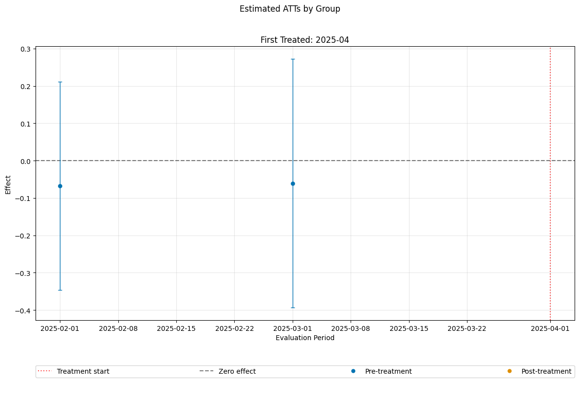
The summary displays estimates of the \(ATT(g,t_\text{eval})\) effects for different combinations of \((g,t_\text{eval})\) via \(\widehat{ATT}(\mathrm{g},t_\text{pre},t_\text{eval})\), where
\(\mathrm{g}\) specifies the group
\(t_\text{pre}\) specifies the corresponding pre-treatment period
\(t_\text{eval}\) specifies the evaluation period
The choice gt_combinations="standard", used estimates all possible combinations of \(ATT(g,t_\text{eval})\) via \(\widehat{ATT}(\mathrm{g},t_\text{pre},t_\text{eval})\), where the standard choice is \(t_\text{pre} = \min(\mathrm{g}, t_\text{eval}) - 1\) (without anticipation).
Remark that this includes pre-tests effects if \(\mathrm{g} > t_{eval}\), e.g. \(\widehat{ATT}(g=\text{2025-04}, t_{\text{pre}}=\text{2025-01}, t_{\text{eval}}=\text{2025-02})\) which estimates the pre-trend from January to February even if the actual treatment occured in April.
As usual for the DoubleML-package, you can obtain joint confidence intervals via bootstrap.
[13]:
level = 0.95

ci = dml_obj.confint(level=level)
dml_obj.bootstrap(n_rep_boot=5000)
ci_joint = dml_obj.confint(level=level, joint=True)
ci_joint
[13]:
| 2.5 % | 97.5 % | |
|---|---|---|
| ATT(2025-04,2025-01,2025-02) | -0.370278 | 0.215010 |
| ATT(2025-04,2025-02,2025-03) | -0.478965 | 0.237199 |
| ATT(2025-04,2025-03,2025-04) | 0.567202 | 1.221488 |
| ATT(2025-04,2025-03,2025-05) | 1.242996 | 2.348027 |
| ATT(2025-04,2025-03,2025-06) | 1.751511 | 3.207124 |
| ATT(2025-05,2025-01,2025-02) | -0.445510 | 0.105945 |
| ATT(2025-05,2025-02,2025-03) | -0.446117 | 0.206877 |
| ATT(2025-05,2025-03,2025-04) | -0.425988 | 0.160946 |
| ATT(2025-05,2025-04,2025-05) | 0.682575 | 1.273216 |
| ATT(2025-05,2025-04,2025-06) | 1.353571 | 2.242616 |
| ATT(2025-06,2025-01,2025-02) | -0.212105 | 0.279638 |
| ATT(2025-06,2025-02,2025-03) | -0.253091 | 0.265926 |
| ATT(2025-06,2025-03,2025-04) | -0.276251 | 0.248381 |
| ATT(2025-06,2025-04,2025-05) | -0.207974 | 0.266679 |
| ATT(2025-06,2025-05,2025-06) | 0.677356 | 1.207704 |
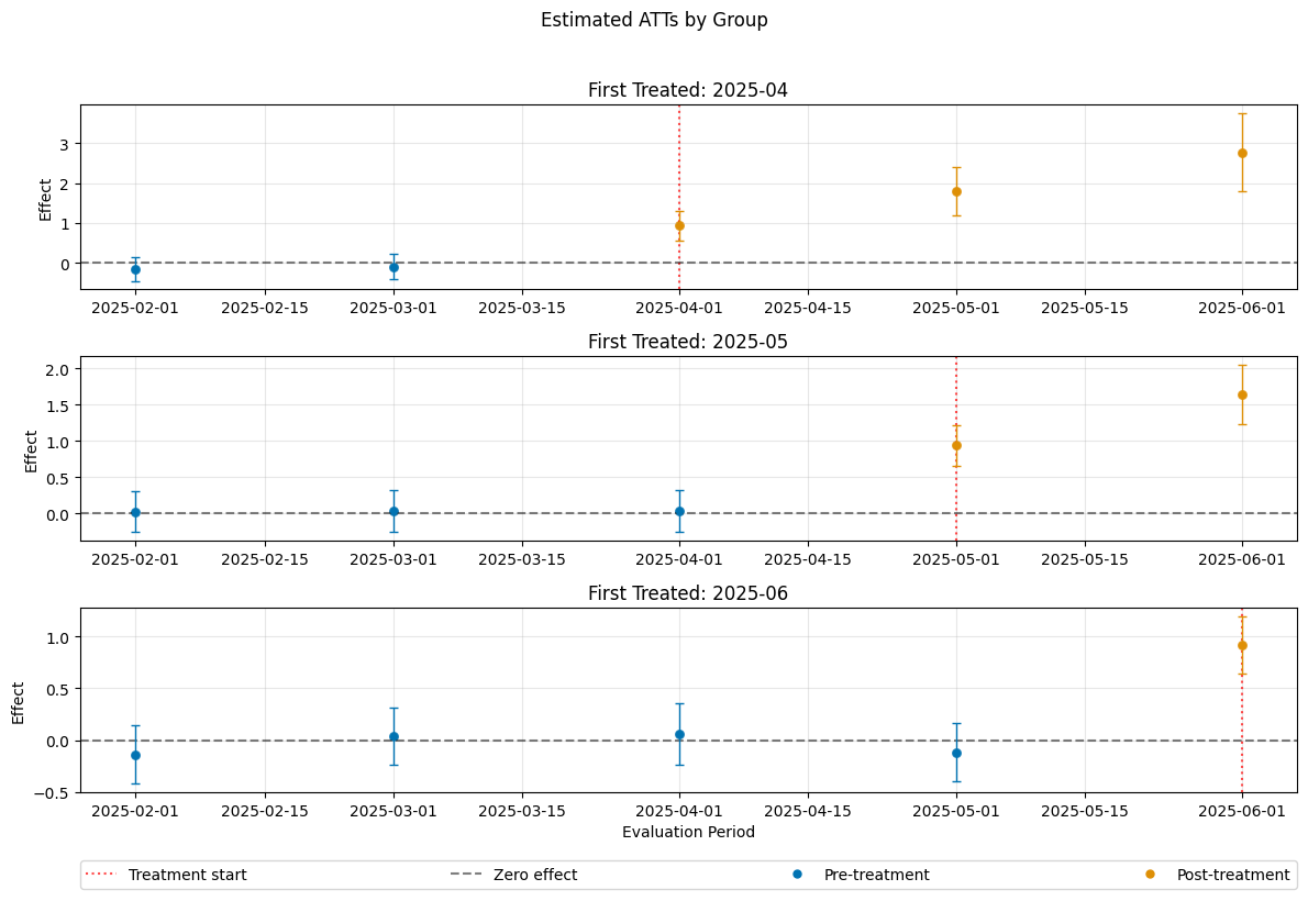
A visualization of the effects can be obtained via the plot_effects() method.
Remark that the plot used joint confidence intervals per default.
[14]:
dml_obj.plot_effects()
[14]:
(<Figure size 1200x800 with 4 Axes>,
 [<Axes: title={'center': 'First Treated: 2025-04'}, ylabel='Effect'>,
  <Axes: title={'center': 'First Treated: 2025-05'}, ylabel='Effect'>,
  <Axes: title={'center': 'First Treated: 2025-06'}, xlabel='Evaluation Period', ylabel='Effect'>])
Sensitivity Analysis#
As descripted in the Sensitivity Guide, robustness checks on omitted confounding/parallel trend violations are available, via the standard sensitivity_analysis() method.
[15]:
dml_obj.sensitivity_analysis()
print(dml_obj.sensitivity_summary)
================== Sensitivity Analysis ==================

------------------ Scenario          ------------------
Significance Level: level=0.95
Sensitivity parameters: cf_y=0.03; cf_d=0.03, rho=1.0

------------------ Bounds with CI    ------------------
                              CI lower  theta lower     theta  theta upper  \
ATT(2025-04,2025-01,2025-02) -0.345875    -0.180627 -0.077634     0.025359
ATT(2025-04,2025-02,2025-03) -0.429566    -0.228382 -0.120883    -0.013383
ATT(2025-04,2025-03,2025-04)  0.611743     0.794804  0.894345     0.993886
ATT(2025-04,2025-03,2025-05)  1.336940     1.644916  1.795511     1.946107
ATT(2025-04,2025-03,2025-06)  1.843625     2.253174  2.479317     2.705461
ATT(2025-05,2025-01,2025-02) -0.425928    -0.271164 -0.169782    -0.068401
ATT(2025-05,2025-02,2025-03) -0.395545    -0.214507 -0.119620    -0.024734
ATT(2025-05,2025-03,2025-04) -0.411534    -0.243900 -0.132521    -0.021142
ATT(2025-05,2025-04,2025-05)  0.708975     0.874958  0.977895     1.080833
ATT(2025-05,2025-04,2025-06)  1.391573     1.642178  1.798093     1.954009
ATT(2025-06,2025-01,2025-02) -0.214552    -0.073338  0.033767     0.140871
ATT(2025-06,2025-02,2025-03) -0.253521    -0.104381  0.006418     0.117217
ATT(2025-06,2025-03,2025-04) -0.270781    -0.120992 -0.013935     0.093122
ATT(2025-06,2025-04,2025-05) -0.212553    -0.076333  0.029352     0.135038
ATT(2025-06,2025-05,2025-06)  0.681592     0.833550  0.942530     1.051510

                              CI upper
ATT(2025-04,2025-01,2025-02)  0.197396
ATT(2025-04,2025-02,2025-03)  0.197641
ATT(2025-04,2025-03,2025-04)  1.188094
ATT(2025-04,2025-03,2025-05)  2.274261
ATT(2025-04,2025-03,2025-06)  3.132882
ATT(2025-05,2025-01,2025-02)  0.094624
ATT(2025-05,2025-02,2025-03)  0.174304
ATT(2025-05,2025-03,2025-04)  0.148672
ATT(2025-05,2025-04,2025-05)  1.254710
ATT(2025-05,2025-04,2025-06)  2.215091
ATT(2025-06,2025-01,2025-02)  0.282282
ATT(2025-06,2025-02,2025-03)  0.266354
ATT(2025-06,2025-03,2025-04)  0.244817
ATT(2025-06,2025-04,2025-05)  0.271641
ATT(2025-06,2025-05,2025-06)  1.204357

------------------ Robustness Values ------------------
                              H_0     RV (%)    RVa (%)
ATT(2025-04,2025-01,2025-02)  0.0   2.269921   0.000342
ATT(2025-04,2025-02,2025-03)  0.0   3.367150   0.000394
ATT(2025-04,2025-03,2025-04)  0.0  23.877860  19.267730
ATT(2025-04,2025-03,2025-05)  0.0  30.316442  25.753034
ATT(2025-04,2025-03,2025-06)  0.0  28.281364  24.363321
ATT(2025-05,2025-01,2025-02)  0.0   4.972732   0.330992
ATT(2025-05,2025-02,2025-03)  0.0   3.767062   0.000593
ATT(2025-05,2025-03,2025-04)  0.0   3.559217   0.000459
ATT(2025-05,2025-04,2025-05)  0.0  25.051670  21.320662
ATT(2025-05,2025-04,2025-06)  0.0  29.496079  25.713224
ATT(2025-06,2025-01,2025-02)  0.0   0.955865   0.000547
ATT(2025-06,2025-02,2025-03)  0.0   0.176126   0.000559
ATT(2025-06,2025-03,2025-04)  0.0   0.395536   0.000554
ATT(2025-06,2025-04,2025-05)  0.0   0.842562   0.000490
ATT(2025-06,2025-05,2025-06)  0.0  23.101698  19.658594
In this example one can clearly, distinguish the robustness of the non-zero effects vs. the pre-treatment periods.
Control Groups#
The current implementation support the following control groups
"never_treated""not_yet_treated"
Remark that the ``”not_yet_treated” depends on anticipation.
For differences and recommendations, we refer to Callaway and Sant’Anna(2021).
[16]:
dml_obj_nyt = DoubleMLDIDMulti(dml_data, **(default_args | {"control_group": "not_yet_treated"}))
dml_obj_nyt.fit()
dml_obj_nyt.bootstrap(n_rep_boot=5000)
dml_obj_nyt.plot_effects()
/opt/hostedtoolcache/Python/3.12.13/x64/lib/python3.12/site-packages/sklearn/utils/validation.py:2739: UserWarning: X does not have valid feature names, but LGBMRegressor was fitted with feature names
  warnings.warn(
/opt/hostedtoolcache/Python/3.12.13/x64/lib/python3.12/site-packages/sklearn/utils/validation.py:2739: UserWarning: X does not have valid feature names, but LGBMRegressor was fitted with feature names
  warnings.warn(
/opt/hostedtoolcache/Python/3.12.13/x64/lib/python3.12/site-packages/sklearn/utils/validation.py:2739: UserWarning: X does not have valid feature names, but LGBMRegressor was fitted with feature names
  warnings.warn(
/opt/hostedtoolcache/Python/3.12.13/x64/lib/python3.12/site-packages/sklearn/utils/validation.py:2739: UserWarning: X does not have valid feature names, but LGBMRegressor was fitted with feature names
  warnings.warn(
/opt/hostedtoolcache/Python/3.12.13/x64/lib/python3.12/site-packages/sklearn/utils/validation.py:2739: UserWarning: X does not have valid feature names, but LGBMRegressor was fitted with feature names
  warnings.warn(
/opt/hostedtoolcache/Python/3.12.13/x64/lib/python3.12/site-packages/sklearn/utils/validation.py:2739: UserWarning: X does not have valid feature names, but LGBMRegressor was fitted with feature names
  warnings.warn(
/opt/hostedtoolcache/Python/3.12.13/x64/lib/python3.12/site-packages/sklearn/utils/validation.py:2739: UserWarning: X does not have valid feature names, but LGBMRegressor was fitted with feature names
  warnings.warn(
/opt/hostedtoolcache/Python/3.12.13/x64/lib/python3.12/site-packages/sklearn/utils/validation.py:2739: UserWarning: X does not have valid feature names, but LGBMRegressor was fitted with feature names
  warnings.warn(
/opt/hostedtoolcache/Python/3.12.13/x64/lib/python3.12/site-packages/sklearn/utils/validation.py:2739: UserWarning: X does not have valid feature names, but LGBMRegressor was fitted with feature names
  warnings.warn(
/opt/hostedtoolcache/Python/3.12.13/x64/lib/python3.12/site-packages/sklearn/utils/validation.py:2739: UserWarning: X does not have valid feature names, but LGBMRegressor was fitted with feature names
  warnings.warn(
/opt/hostedtoolcache/Python/3.12.13/x64/lib/python3.12/site-packages/sklearn/utils/validation.py:2739: UserWarning: X does not have valid feature names, but LGBMClassifier was fitted with feature names
  warnings.warn(
/opt/hostedtoolcache/Python/3.12.13/x64/lib/python3.12/site-packages/sklearn/utils/validation.py:2739: UserWarning: X does not have valid feature names, but LGBMClassifier was fitted with feature names
  warnings.warn(
/opt/hostedtoolcache/Python/3.12.13/x64/lib/python3.12/site-packages/sklearn/utils/validation.py:2739: UserWarning: X does not have valid feature names, but LGBMClassifier was fitted with feature names
  warnings.warn(
/opt/hostedtoolcache/Python/3.12.13/x64/lib/python3.12/site-packages/sklearn/utils/validation.py:2739: UserWarning: X does not have valid feature names, but LGBMClassifier was fitted with feature names
  warnings.warn(
/opt/hostedtoolcache/Python/3.12.13/x64/lib/python3.12/site-packages/sklearn/utils/validation.py:2739: UserWarning: X does not have valid feature names, but LGBMClassifier was fitted with feature names
  warnings.warn(
/opt/hostedtoolcache/Python/3.12.13/x64/lib/python3.12/site-packages/sklearn/utils/validation.py:2739: UserWarning: X does not have valid feature names, but LGBMRegressor was fitted with feature names
  warnings.warn(
/opt/hostedtoolcache/Python/3.12.13/x64/lib/python3.12/site-packages/sklearn/utils/validation.py:2739: UserWarning: X does not have valid feature names, but LGBMRegressor was fitted with feature names
  warnings.warn(
/opt/hostedtoolcache/Python/3.12.13/x64/lib/python3.12/site-packages/sklearn/utils/validation.py:2739: UserWarning: X does not have valid feature names, but LGBMRegressor was fitted with feature names
  warnings.warn(
/opt/hostedtoolcache/Python/3.12.13/x64/lib/python3.12/site-packages/sklearn/utils/validation.py:2739: UserWarning: X does not have valid feature names, but LGBMRegressor was fitted with feature names
  warnings.warn(
/opt/hostedtoolcache/Python/3.12.13/x64/lib/python3.12/site-packages/sklearn/utils/validation.py:2739: UserWarning: X does not have valid feature names, but LGBMRegressor was fitted with feature names
  warnings.warn(
/opt/hostedtoolcache/Python/3.12.13/x64/lib/python3.12/site-packages/sklearn/utils/validation.py:2739: UserWarning: X does not have valid feature names, but LGBMRegressor was fitted with feature names
  warnings.warn(
/opt/hostedtoolcache/Python/3.12.13/x64/lib/python3.12/site-packages/sklearn/utils/validation.py:2739: UserWarning: X does not have valid feature names, but LGBMRegressor was fitted with feature names
  warnings.warn(
/opt/hostedtoolcache/Python/3.12.13/x64/lib/python3.12/site-packages/sklearn/utils/validation.py:2739: UserWarning: X does not have valid feature names, but LGBMRegressor was fitted with feature names
  warnings.warn(
/opt/hostedtoolcache/Python/3.12.13/x64/lib/python3.12/site-packages/sklearn/utils/validation.py:2739: UserWarning: X does not have valid feature names, but LGBMRegressor was fitted with feature names
  warnings.warn(
/opt/hostedtoolcache/Python/3.12.13/x64/lib/python3.12/site-packages/sklearn/utils/validation.py:2739: UserWarning: X does not have valid feature names, but LGBMRegressor was fitted with feature names
  warnings.warn(
/opt/hostedtoolcache/Python/3.12.13/x64/lib/python3.12/site-packages/sklearn/utils/validation.py:2739: UserWarning: X does not have valid feature names, but LGBMClassifier was fitted with feature names
  warnings.warn(
/opt/hostedtoolcache/Python/3.12.13/x64/lib/python3.12/site-packages/sklearn/utils/validation.py:2739: UserWarning: X does not have valid feature names, but LGBMClassifier was fitted with feature names
  warnings.warn(
/opt/hostedtoolcache/Python/3.12.13/x64/lib/python3.12/site-packages/sklearn/utils/validation.py:2739: UserWarning: X does not have valid feature names, but LGBMClassifier was fitted with feature names
  warnings.warn(
/opt/hostedtoolcache/Python/3.12.13/x64/lib/python3.12/site-packages/sklearn/utils/validation.py:2739: UserWarning: X does not have valid feature names, but LGBMClassifier was fitted with feature names
  warnings.warn(
/opt/hostedtoolcache/Python/3.12.13/x64/lib/python3.12/site-packages/sklearn/utils/validation.py:2739: UserWarning: X does not have valid feature names, but LGBMClassifier was fitted with feature names
  warnings.warn(
/opt/hostedtoolcache/Python/3.12.13/x64/lib/python3.12/site-packages/sklearn/utils/validation.py:2739: UserWarning: X does not have valid feature names, but LGBMRegressor was fitted with feature names
  warnings.warn(
/opt/hostedtoolcache/Python/3.12.13/x64/lib/python3.12/site-packages/sklearn/utils/validation.py:2739: UserWarning: X does not have valid feature names, but LGBMRegressor was fitted with feature names
  warnings.warn(
/opt/hostedtoolcache/Python/3.12.13/x64/lib/python3.12/site-packages/sklearn/utils/validation.py:2739: UserWarning: X does not have valid feature names, but LGBMRegressor was fitted with feature names
  warnings.warn(
/opt/hostedtoolcache/Python/3.12.13/x64/lib/python3.12/site-packages/sklearn/utils/validation.py:2739: UserWarning: X does not have valid feature names, but LGBMRegressor was fitted with feature names
  warnings.warn(
/opt/hostedtoolcache/Python/3.12.13/x64/lib/python3.12/site-packages/sklearn/utils/validation.py:2739: UserWarning: X does not have valid feature names, but LGBMRegressor was fitted with feature names
  warnings.warn(
/opt/hostedtoolcache/Python/3.12.13/x64/lib/python3.12/site-packages/sklearn/utils/validation.py:2739: UserWarning: X does not have valid feature names, but LGBMRegressor was fitted with feature names
  warnings.warn(
/opt/hostedtoolcache/Python/3.12.13/x64/lib/python3.12/site-packages/sklearn/utils/validation.py:2739: UserWarning: X does not have valid feature names, but LGBMRegressor was fitted with feature names
  warnings.warn(
/opt/hostedtoolcache/Python/3.12.13/x64/lib/python3.12/site-packages/sklearn/utils/validation.py:2739: UserWarning: X does not have valid feature names, but LGBMRegressor was fitted with feature names
  warnings.warn(
/opt/hostedtoolcache/Python/3.12.13/x64/lib/python3.12/site-packages/sklearn/utils/validation.py:2739: UserWarning: X does not have valid feature names, but LGBMRegressor was fitted with feature names
  warnings.warn(
/opt/hostedtoolcache/Python/3.12.13/x64/lib/python3.12/site-packages/sklearn/utils/validation.py:2739: UserWarning: X does not have valid feature names, but LGBMRegressor was fitted with feature names
  warnings.warn(
/opt/hostedtoolcache/Python/3.12.13/x64/lib/python3.12/site-packages/sklearn/utils/validation.py:2739: UserWarning: X does not have valid feature names, but LGBMClassifier was fitted with feature names
  warnings.warn(
/opt/hostedtoolcache/Python/3.12.13/x64/lib/python3.12/site-packages/sklearn/utils/validation.py:2739: UserWarning: X does not have valid feature names, but LGBMClassifier was fitted with feature names
  warnings.warn(
/opt/hostedtoolcache/Python/3.12.13/x64/lib/python3.12/site-packages/sklearn/utils/validation.py:2739: UserWarning: X does not have valid feature names, but LGBMClassifier was fitted with feature names
  warnings.warn(
/opt/hostedtoolcache/Python/3.12.13/x64/lib/python3.12/site-packages/sklearn/utils/validation.py:2739: UserWarning: X does not have valid feature names, but LGBMClassifier was fitted with feature names
  warnings.warn(
/opt/hostedtoolcache/Python/3.12.13/x64/lib/python3.12/site-packages/sklearn/utils/validation.py:2739: UserWarning: X does not have valid feature names, but LGBMClassifier was fitted with feature names
  warnings.warn(
/opt/hostedtoolcache/Python/3.12.13/x64/lib/python3.12/site-packages/sklearn/utils/validation.py:2739: UserWarning: X does not have valid feature names, but LGBMRegressor was fitted with feature names
  warnings.warn(
/opt/hostedtoolcache/Python/3.12.13/x64/lib/python3.12/site-packages/sklearn/utils/validation.py:2739: UserWarning: X does not have valid feature names, but LGBMRegressor was fitted with feature names
  warnings.warn(
/opt/hostedtoolcache/Python/3.12.13/x64/lib/python3.12/site-packages/sklearn/utils/validation.py:2739: UserWarning: X does not have valid feature names, but LGBMRegressor was fitted with feature names
  warnings.warn(
/opt/hostedtoolcache/Python/3.12.13/x64/lib/python3.12/site-packages/sklearn/utils/validation.py:2739: UserWarning: X does not have valid feature names, but LGBMRegressor was fitted with feature names
  warnings.warn(
/opt/hostedtoolcache/Python/3.12.13/x64/lib/python3.12/site-packages/sklearn/utils/validation.py:2739: UserWarning: X does not have valid feature names, but LGBMRegressor was fitted with feature names
  warnings.warn(
/opt/hostedtoolcache/Python/3.12.13/x64/lib/python3.12/site-packages/sklearn/utils/validation.py:2739: UserWarning: X does not have valid feature names, but LGBMRegressor was fitted with feature names
  warnings.warn(
/opt/hostedtoolcache/Python/3.12.13/x64/lib/python3.12/site-packages/sklearn/utils/validation.py:2739: UserWarning: X does not have valid feature names, but LGBMRegressor was fitted with feature names
  warnings.warn(
/opt/hostedtoolcache/Python/3.12.13/x64/lib/python3.12/site-packages/sklearn/utils/validation.py:2739: UserWarning: X does not have valid feature names, but LGBMRegressor was fitted with feature names
  warnings.warn(
/opt/hostedtoolcache/Python/3.12.13/x64/lib/python3.12/site-packages/sklearn/utils/validation.py:2739: UserWarning: X does not have valid feature names, but LGBMRegressor was fitted with feature names
  warnings.warn(
/opt/hostedtoolcache/Python/3.12.13/x64/lib/python3.12/site-packages/sklearn/utils/validation.py:2739: UserWarning: X does not have valid feature names, but LGBMRegressor was fitted with feature names
  warnings.warn(
/opt/hostedtoolcache/Python/3.12.13/x64/lib/python3.12/site-packages/sklearn/utils/validation.py:2739: UserWarning: X does not have valid feature names, but LGBMClassifier was fitted with feature names
  warnings.warn(
/opt/hostedtoolcache/Python/3.12.13/x64/lib/python3.12/site-packages/sklearn/utils/validation.py:2739: UserWarning: X does not have valid feature names, but LGBMClassifier was fitted with feature names
  warnings.warn(
/opt/hostedtoolcache/Python/3.12.13/x64/lib/python3.12/site-packages/sklearn/utils/validation.py:2739: UserWarning: X does not have valid feature names, but LGBMClassifier was fitted with feature names
  warnings.warn(
/opt/hostedtoolcache/Python/3.12.13/x64/lib/python3.12/site-packages/sklearn/utils/validation.py:2739: UserWarning: X does not have valid feature names, but LGBMClassifier was fitted with feature names
  warnings.warn(
/opt/hostedtoolcache/Python/3.12.13/x64/lib/python3.12/site-packages/sklearn/utils/validation.py:2739: UserWarning: X does not have valid feature names, but LGBMClassifier was fitted with feature names
  warnings.warn(
/opt/hostedtoolcache/Python/3.12.13/x64/lib/python3.12/site-packages/sklearn/utils/validation.py:2739: UserWarning: X does not have valid feature names, but LGBMRegressor was fitted with feature names
  warnings.warn(
/opt/hostedtoolcache/Python/3.12.13/x64/lib/python3.12/site-packages/sklearn/utils/validation.py:2739: UserWarning: X does not have valid feature names, but LGBMRegressor was fitted with feature names
  warnings.warn(
/opt/hostedtoolcache/Python/3.12.13/x64/lib/python3.12/site-packages/sklearn/utils/validation.py:2739: UserWarning: X does not have valid feature names, but LGBMRegressor was fitted with feature names
  warnings.warn(
/opt/hostedtoolcache/Python/3.12.13/x64/lib/python3.12/site-packages/sklearn/utils/validation.py:2739: UserWarning: X does not have valid feature names, but LGBMRegressor was fitted with feature names
  warnings.warn(
/opt/hostedtoolcache/Python/3.12.13/x64/lib/python3.12/site-packages/sklearn/utils/validation.py:2739: UserWarning: X does not have valid feature names, but LGBMRegressor was fitted with feature names
  warnings.warn(
/opt/hostedtoolcache/Python/3.12.13/x64/lib/python3.12/site-packages/sklearn/utils/validation.py:2739: UserWarning: X does not have valid feature names, but LGBMRegressor was fitted with feature names
  warnings.warn(
/opt/hostedtoolcache/Python/3.12.13/x64/lib/python3.12/site-packages/sklearn/utils/validation.py:2739: UserWarning: X does not have valid feature names, but LGBMRegressor was fitted with feature names
  warnings.warn(
/opt/hostedtoolcache/Python/3.12.13/x64/lib/python3.12/site-packages/sklearn/utils/validation.py:2739: UserWarning: X does not have valid feature names, but LGBMRegressor was fitted with feature names
  warnings.warn(
/opt/hostedtoolcache/Python/3.12.13/x64/lib/python3.12/site-packages/sklearn/utils/validation.py:2739: UserWarning: X does not have valid feature names, but LGBMRegressor was fitted with feature names
  warnings.warn(
/opt/hostedtoolcache/Python/3.12.13/x64/lib/python3.12/site-packages/sklearn/utils/validation.py:2739: UserWarning: X does not have valid feature names, but LGBMRegressor was fitted with feature names
  warnings.warn(
/opt/hostedtoolcache/Python/3.12.13/x64/lib/python3.12/site-packages/sklearn/utils/validation.py:2739: UserWarning: X does not have valid feature names, but LGBMClassifier was fitted with feature names
  warnings.warn(
/opt/hostedtoolcache/Python/3.12.13/x64/lib/python3.12/site-packages/sklearn/utils/validation.py:2739: UserWarning: X does not have valid feature names, but LGBMClassifier was fitted with feature names
  warnings.warn(
/opt/hostedtoolcache/Python/3.12.13/x64/lib/python3.12/site-packages/sklearn/utils/validation.py:2739: UserWarning: X does not have valid feature names, but LGBMClassifier was fitted with feature names
  warnings.warn(
/opt/hostedtoolcache/Python/3.12.13/x64/lib/python3.12/site-packages/sklearn/utils/validation.py:2739: UserWarning: X does not have valid feature names, but LGBMClassifier was fitted with feature names
  warnings.warn(
/opt/hostedtoolcache/Python/3.12.13/x64/lib/python3.12/site-packages/sklearn/utils/validation.py:2739: UserWarning: X does not have valid feature names, but LGBMClassifier was fitted with feature names
  warnings.warn(
/opt/hostedtoolcache/Python/3.12.13/x64/lib/python3.12/site-packages/sklearn/utils/validation.py:2739: UserWarning: X does not have valid feature names, but LGBMRegressor was fitted with feature names
  warnings.warn(
/opt/hostedtoolcache/Python/3.12.13/x64/lib/python3.12/site-packages/sklearn/utils/validation.py:2739: UserWarning: X does not have valid feature names, but LGBMRegressor was fitted with feature names
  warnings.warn(
/opt/hostedtoolcache/Python/3.12.13/x64/lib/python3.12/site-packages/sklearn/utils/validation.py:2739: UserWarning: X does not have valid feature names, but LGBMRegressor was fitted with feature names
  warnings.warn(
/opt/hostedtoolcache/Python/3.12.13/x64/lib/python3.12/site-packages/sklearn/utils/validation.py:2739: UserWarning: X does not have valid feature names, but LGBMRegressor was fitted with feature names
  warnings.warn(
/opt/hostedtoolcache/Python/3.12.13/x64/lib/python3.12/site-packages/sklearn/utils/validation.py:2739: UserWarning: X does not have valid feature names, but LGBMRegressor was fitted with feature names
  warnings.warn(
/opt/hostedtoolcache/Python/3.12.13/x64/lib/python3.12/site-packages/sklearn/utils/validation.py:2739: UserWarning: X does not have valid feature names, but LGBMRegressor was fitted with feature names
  warnings.warn(
/opt/hostedtoolcache/Python/3.12.13/x64/lib/python3.12/site-packages/sklearn/utils/validation.py:2739: UserWarning: X does not have valid feature names, but LGBMRegressor was fitted with feature names
  warnings.warn(
/opt/hostedtoolcache/Python/3.12.13/x64/lib/python3.12/site-packages/sklearn/utils/validation.py:2739: UserWarning: X does not have valid feature names, but LGBMRegressor was fitted with feature names
  warnings.warn(
/opt/hostedtoolcache/Python/3.12.13/x64/lib/python3.12/site-packages/sklearn/utils/validation.py:2739: UserWarning: X does not have valid feature names, but LGBMRegressor was fitted with feature names
  warnings.warn(
/opt/hostedtoolcache/Python/3.12.13/x64/lib/python3.12/site-packages/sklearn/utils/validation.py:2739: UserWarning: X does not have valid feature names, but LGBMRegressor was fitted with feature names
  warnings.warn(
/opt/hostedtoolcache/Python/3.12.13/x64/lib/python3.12/site-packages/sklearn/utils/validation.py:2739: UserWarning: X does not have valid feature names, but LGBMClassifier was fitted with feature names
  warnings.warn(
/opt/hostedtoolcache/Python/3.12.13/x64/lib/python3.12/site-packages/sklearn/utils/validation.py:2739: UserWarning: X does not have valid feature names, but LGBMClassifier was fitted with feature names
  warnings.warn(
/opt/hostedtoolcache/Python/3.12.13/x64/lib/python3.12/site-packages/sklearn/utils/validation.py:2739: UserWarning: X does not have valid feature names, but LGBMClassifier was fitted with feature names
  warnings.warn(
/opt/hostedtoolcache/Python/3.12.13/x64/lib/python3.12/site-packages/sklearn/utils/validation.py:2739: UserWarning: X does not have valid feature names, but LGBMClassifier was fitted with feature names
  warnings.warn(
/opt/hostedtoolcache/Python/3.12.13/x64/lib/python3.12/site-packages/sklearn/utils/validation.py:2739: UserWarning: X does not have valid feature names, but LGBMClassifier was fitted with feature names
  warnings.warn(
/opt/hostedtoolcache/Python/3.12.13/x64/lib/python3.12/site-packages/sklearn/utils/validation.py:2739: UserWarning: X does not have valid feature names, but LGBMRegressor was fitted with feature names
  warnings.warn(
/opt/hostedtoolcache/Python/3.12.13/x64/lib/python3.12/site-packages/sklearn/utils/validation.py:2739: UserWarning: X does not have valid feature names, but LGBMRegressor was fitted with feature names
  warnings.warn(
/opt/hostedtoolcache/Python/3.12.13/x64/lib/python3.12/site-packages/sklearn/utils/validation.py:2739: UserWarning: X does not have valid feature names, but LGBMRegressor was fitted with feature names
  warnings.warn(
/opt/hostedtoolcache/Python/3.12.13/x64/lib/python3.12/site-packages/sklearn/utils/validation.py:2739: UserWarning: X does not have valid feature names, but LGBMRegressor was fitted with feature names
  warnings.warn(
/opt/hostedtoolcache/Python/3.12.13/x64/lib/python3.12/site-packages/sklearn/utils/validation.py:2739: UserWarning: X does not have valid feature names, but LGBMRegressor was fitted with feature names
  warnings.warn(
/opt/hostedtoolcache/Python/3.12.13/x64/lib/python3.12/site-packages/sklearn/utils/validation.py:2739: UserWarning: X does not have valid feature names, but LGBMRegressor was fitted with feature names
  warnings.warn(
/opt/hostedtoolcache/Python/3.12.13/x64/lib/python3.12/site-packages/sklearn/utils/validation.py:2739: UserWarning: X does not have valid feature names, but LGBMRegressor was fitted with feature names
  warnings.warn(
/opt/hostedtoolcache/Python/3.12.13/x64/lib/python3.12/site-packages/sklearn/utils/validation.py:2739: UserWarning: X does not have valid feature names, but LGBMRegressor was fitted with feature names
  warnings.warn(
/opt/hostedtoolcache/Python/3.12.13/x64/lib/python3.12/site-packages/sklearn/utils/validation.py:2739: UserWarning: X does not have valid feature names, but LGBMRegressor was fitted with feature names
  warnings.warn(
/opt/hostedtoolcache/Python/3.12.13/x64/lib/python3.12/site-packages/sklearn/utils/validation.py:2739: UserWarning: X does not have valid feature names, but LGBMRegressor was fitted with feature names
  warnings.warn(
/opt/hostedtoolcache/Python/3.12.13/x64/lib/python3.12/site-packages/sklearn/utils/validation.py:2739: UserWarning: X does not have valid feature names, but LGBMClassifier was fitted with feature names
  warnings.warn(
/opt/hostedtoolcache/Python/3.12.13/x64/lib/python3.12/site-packages/sklearn/utils/validation.py:2739: UserWarning: X does not have valid feature names, but LGBMClassifier was fitted with feature names
  warnings.warn(
/opt/hostedtoolcache/Python/3.12.13/x64/lib/python3.12/site-packages/sklearn/utils/validation.py:2739: UserWarning: X does not have valid feature names, but LGBMClassifier was fitted with feature names
  warnings.warn(
/opt/hostedtoolcache/Python/3.12.13/x64/lib/python3.12/site-packages/sklearn/utils/validation.py:2739: UserWarning: X does not have valid feature names, but LGBMClassifier was fitted with feature names
  warnings.warn(
/opt/hostedtoolcache/Python/3.12.13/x64/lib/python3.12/site-packages/sklearn/utils/validation.py:2739: UserWarning: X does not have valid feature names, but LGBMClassifier was fitted with feature names
  warnings.warn(
/opt/hostedtoolcache/Python/3.12.13/x64/lib/python3.12/site-packages/sklearn/utils/validation.py:2739: UserWarning: X does not have valid feature names, but LGBMRegressor was fitted with feature names
  warnings.warn(
/opt/hostedtoolcache/Python/3.12.13/x64/lib/python3.12/site-packages/sklearn/utils/validation.py:2739: UserWarning: X does not have valid feature names, but LGBMRegressor was fitted with feature names
  warnings.warn(
/opt/hostedtoolcache/Python/3.12.13/x64/lib/python3.12/site-packages/sklearn/utils/validation.py:2739: UserWarning: X does not have valid feature names, but LGBMRegressor was fitted with feature names
  warnings.warn(
/opt/hostedtoolcache/Python/3.12.13/x64/lib/python3.12/site-packages/sklearn/utils/validation.py:2739: UserWarning: X does not have valid feature names, but LGBMRegressor was fitted with feature names
  warnings.warn(
/opt/hostedtoolcache/Python/3.12.13/x64/lib/python3.12/site-packages/sklearn/utils/validation.py:2739: UserWarning: X does not have valid feature names, but LGBMRegressor was fitted with feature names
  warnings.warn(
/opt/hostedtoolcache/Python/3.12.13/x64/lib/python3.12/site-packages/sklearn/utils/validation.py:2739: UserWarning: X does not have valid feature names, but LGBMRegressor was fitted with feature names
  warnings.warn(
/opt/hostedtoolcache/Python/3.12.13/x64/lib/python3.12/site-packages/sklearn/utils/validation.py:2739: UserWarning: X does not have valid feature names, but LGBMRegressor was fitted with feature names
  warnings.warn(
/opt/hostedtoolcache/Python/3.12.13/x64/lib/python3.12/site-packages/sklearn/utils/validation.py:2739: UserWarning: X does not have valid feature names, but LGBMRegressor was fitted with feature names
  warnings.warn(
/opt/hostedtoolcache/Python/3.12.13/x64/lib/python3.12/site-packages/sklearn/utils/validation.py:2739: UserWarning: X does not have valid feature names, but LGBMRegressor was fitted with feature names
  warnings.warn(
/opt/hostedtoolcache/Python/3.12.13/x64/lib/python3.12/site-packages/sklearn/utils/validation.py:2739: UserWarning: X does not have valid feature names, but LGBMRegressor was fitted with feature names
  warnings.warn(
/opt/hostedtoolcache/Python/3.12.13/x64/lib/python3.12/site-packages/sklearn/utils/validation.py:2739: UserWarning: X does not have valid feature names, but LGBMClassifier was fitted with feature names
  warnings.warn(
/opt/hostedtoolcache/Python/3.12.13/x64/lib/python3.12/site-packages/sklearn/utils/validation.py:2739: UserWarning: X does not have valid feature names, but LGBMClassifier was fitted with feature names
  warnings.warn(
/opt/hostedtoolcache/Python/3.12.13/x64/lib/python3.12/site-packages/sklearn/utils/validation.py:2739: UserWarning: X does not have valid feature names, but LGBMClassifier was fitted with feature names
  warnings.warn(
/opt/hostedtoolcache/Python/3.12.13/x64/lib/python3.12/site-packages/sklearn/utils/validation.py:2739: UserWarning: X does not have valid feature names, but LGBMClassifier was fitted with feature names
  warnings.warn(
/opt/hostedtoolcache/Python/3.12.13/x64/lib/python3.12/site-packages/sklearn/utils/validation.py:2739: UserWarning: X does not have valid feature names, but LGBMClassifier was fitted with feature names
  warnings.warn(
/opt/hostedtoolcache/Python/3.12.13/x64/lib/python3.12/site-packages/sklearn/utils/validation.py:2739: UserWarning: X does not have valid feature names, but LGBMRegressor was fitted with feature names
  warnings.warn(
/opt/hostedtoolcache/Python/3.12.13/x64/lib/python3.12/site-packages/sklearn/utils/validation.py:2739: UserWarning: X does not have valid feature names, but LGBMRegressor was fitted with feature names
  warnings.warn(
/opt/hostedtoolcache/Python/3.12.13/x64/lib/python3.12/site-packages/sklearn/utils/validation.py:2739: UserWarning: X does not have valid feature names, but LGBMRegressor was fitted with feature names
  warnings.warn(
/opt/hostedtoolcache/Python/3.12.13/x64/lib/python3.12/site-packages/sklearn/utils/validation.py:2739: UserWarning: X does not have valid feature names, but LGBMRegressor was fitted with feature names
  warnings.warn(
/opt/hostedtoolcache/Python/3.12.13/x64/lib/python3.12/site-packages/sklearn/utils/validation.py:2739: UserWarning: X does not have valid feature names, but LGBMRegressor was fitted with feature names
  warnings.warn(
/opt/hostedtoolcache/Python/3.12.13/x64/lib/python3.12/site-packages/sklearn/utils/validation.py:2739: UserWarning: X does not have valid feature names, but LGBMRegressor was fitted with feature names
  warnings.warn(
/opt/hostedtoolcache/Python/3.12.13/x64/lib/python3.12/site-packages/sklearn/utils/validation.py:2739: UserWarning: X does not have valid feature names, but LGBMRegressor was fitted with feature names
  warnings.warn(
/opt/hostedtoolcache/Python/3.12.13/x64/lib/python3.12/site-packages/sklearn/utils/validation.py:2739: UserWarning: X does not have valid feature names, but LGBMRegressor was fitted with feature names
  warnings.warn(
/opt/hostedtoolcache/Python/3.12.13/x64/lib/python3.12/site-packages/sklearn/utils/validation.py:2739: UserWarning: X does not have valid feature names, but LGBMRegressor was fitted with feature names
  warnings.warn(
/opt/hostedtoolcache/Python/3.12.13/x64/lib/python3.12/site-packages/sklearn/utils/validation.py:2739: UserWarning: X does not have valid feature names, but LGBMRegressor was fitted with feature names
  warnings.warn(
/opt/hostedtoolcache/Python/3.12.13/x64/lib/python3.12/site-packages/sklearn/utils/validation.py:2739: UserWarning: X does not have valid feature names, but LGBMClassifier was fitted with feature names
  warnings.warn(
/opt/hostedtoolcache/Python/3.12.13/x64/lib/python3.12/site-packages/sklearn/utils/validation.py:2739: UserWarning: X does not have valid feature names, but LGBMClassifier was fitted with feature names
  warnings.warn(
/opt/hostedtoolcache/Python/3.12.13/x64/lib/python3.12/site-packages/sklearn/utils/validation.py:2739: UserWarning: X does not have valid feature names, but LGBMClassifier was fitted with feature names
  warnings.warn(
/opt/hostedtoolcache/Python/3.12.13/x64/lib/python3.12/site-packages/sklearn/utils/validation.py:2739: UserWarning: X does not have valid feature names, but LGBMClassifier was fitted with feature names
  warnings.warn(
/opt/hostedtoolcache/Python/3.12.13/x64/lib/python3.12/site-packages/sklearn/utils/validation.py:2739: UserWarning: X does not have valid feature names, but LGBMClassifier was fitted with feature names
  warnings.warn(
/opt/hostedtoolcache/Python/3.12.13/x64/lib/python3.12/site-packages/sklearn/utils/validation.py:2739: UserWarning: X does not have valid feature names, but LGBMRegressor was fitted with feature names
  warnings.warn(
/opt/hostedtoolcache/Python/3.12.13/x64/lib/python3.12/site-packages/sklearn/utils/validation.py:2739: UserWarning: X does not have valid feature names, but LGBMRegressor was fitted with feature names
  warnings.warn(
/opt/hostedtoolcache/Python/3.12.13/x64/lib/python3.12/site-packages/sklearn/utils/validation.py:2739: UserWarning: X does not have valid feature names, but LGBMRegressor was fitted with feature names
  warnings.warn(
/opt/hostedtoolcache/Python/3.12.13/x64/lib/python3.12/site-packages/sklearn/utils/validation.py:2739: UserWarning: X does not have valid feature names, but LGBMRegressor was fitted with feature names
  warnings.warn(
/opt/hostedtoolcache/Python/3.12.13/x64/lib/python3.12/site-packages/sklearn/utils/validation.py:2739: UserWarning: X does not have valid feature names, but LGBMRegressor was fitted with feature names
  warnings.warn(
/opt/hostedtoolcache/Python/3.12.13/x64/lib/python3.12/site-packages/sklearn/utils/validation.py:2739: UserWarning: X does not have valid feature names, but LGBMRegressor was fitted with feature names
  warnings.warn(
/opt/hostedtoolcache/Python/3.12.13/x64/lib/python3.12/site-packages/sklearn/utils/validation.py:2739: UserWarning: X does not have valid feature names, but LGBMRegressor was fitted with feature names
  warnings.warn(
/opt/hostedtoolcache/Python/3.12.13/x64/lib/python3.12/site-packages/sklearn/utils/validation.py:2739: UserWarning: X does not have valid feature names, but LGBMRegressor was fitted with feature names
  warnings.warn(
/opt/hostedtoolcache/Python/3.12.13/x64/lib/python3.12/site-packages/sklearn/utils/validation.py:2739: UserWarning: X does not have valid feature names, but LGBMRegressor was fitted with feature names
  warnings.warn(
/opt/hostedtoolcache/Python/3.12.13/x64/lib/python3.12/site-packages/sklearn/utils/validation.py:2739: UserWarning: X does not have valid feature names, but LGBMRegressor was fitted with feature names
  warnings.warn(
/opt/hostedtoolcache/Python/3.12.13/x64/lib/python3.12/site-packages/sklearn/utils/validation.py:2739: UserWarning: X does not have valid feature names, but LGBMClassifier was fitted with feature names
  warnings.warn(
/opt/hostedtoolcache/Python/3.12.13/x64/lib/python3.12/site-packages/sklearn/utils/validation.py:2739: UserWarning: X does not have valid feature names, but LGBMClassifier was fitted with feature names
  warnings.warn(
/opt/hostedtoolcache/Python/3.12.13/x64/lib/python3.12/site-packages/sklearn/utils/validation.py:2739: UserWarning: X does not have valid feature names, but LGBMClassifier was fitted with feature names
  warnings.warn(
/opt/hostedtoolcache/Python/3.12.13/x64/lib/python3.12/site-packages/sklearn/utils/validation.py:2739: UserWarning: X does not have valid feature names, but LGBMClassifier was fitted with feature names
  warnings.warn(
/opt/hostedtoolcache/Python/3.12.13/x64/lib/python3.12/site-packages/sklearn/utils/validation.py:2739: UserWarning: X does not have valid feature names, but LGBMClassifier was fitted with feature names
  warnings.warn(
/opt/hostedtoolcache/Python/3.12.13/x64/lib/python3.12/site-packages/sklearn/utils/validation.py:2739: UserWarning: X does not have valid feature names, but LGBMRegressor was fitted with feature names
  warnings.warn(
/opt/hostedtoolcache/Python/3.12.13/x64/lib/python3.12/site-packages/sklearn/utils/validation.py:2739: UserWarning: X does not have valid feature names, but LGBMRegressor was fitted with feature names
  warnings.warn(
/opt/hostedtoolcache/Python/3.12.13/x64/lib/python3.12/site-packages/sklearn/utils/validation.py:2739: UserWarning: X does not have valid feature names, but LGBMRegressor was fitted with feature names
  warnings.warn(
/opt/hostedtoolcache/Python/3.12.13/x64/lib/python3.12/site-packages/sklearn/utils/validation.py:2739: UserWarning: X does not have valid feature names, but LGBMRegressor was fitted with feature names
  warnings.warn(
/opt/hostedtoolcache/Python/3.12.13/x64/lib/python3.12/site-packages/sklearn/utils/validation.py:2739: UserWarning: X does not have valid feature names, but LGBMRegressor was fitted with feature names
  warnings.warn(
/opt/hostedtoolcache/Python/3.12.13/x64/lib/python3.12/site-packages/sklearn/utils/validation.py:2739: UserWarning: X does not have valid feature names, but LGBMRegressor was fitted with feature names
  warnings.warn(
/opt/hostedtoolcache/Python/3.12.13/x64/lib/python3.12/site-packages/sklearn/utils/validation.py:2739: UserWarning: X does not have valid feature names, but LGBMRegressor was fitted with feature names
  warnings.warn(
/opt/hostedtoolcache/Python/3.12.13/x64/lib/python3.12/site-packages/sklearn/utils/validation.py:2739: UserWarning: X does not have valid feature names, but LGBMRegressor was fitted with feature names
  warnings.warn(
/opt/hostedtoolcache/Python/3.12.13/x64/lib/python3.12/site-packages/sklearn/utils/validation.py:2739: UserWarning: X does not have valid feature names, but LGBMRegressor was fitted with feature names
  warnings.warn(
/opt/hostedtoolcache/Python/3.12.13/x64/lib/python3.12/site-packages/sklearn/utils/validation.py:2739: UserWarning: X does not have valid feature names, but LGBMRegressor was fitted with feature names
  warnings.warn(
/opt/hostedtoolcache/Python/3.12.13/x64/lib/python3.12/site-packages/sklearn/utils/validation.py:2739: UserWarning: X does not have valid feature names, but LGBMClassifier was fitted with feature names
  warnings.warn(
/opt/hostedtoolcache/Python/3.12.13/x64/lib/python3.12/site-packages/sklearn/utils/validation.py:2739: UserWarning: X does not have valid feature names, but LGBMClassifier was fitted with feature names
  warnings.warn(
/opt/hostedtoolcache/Python/3.12.13/x64/lib/python3.12/site-packages/sklearn/utils/validation.py:2739: UserWarning: X does not have valid feature names, but LGBMClassifier was fitted with feature names
  warnings.warn(
/opt/hostedtoolcache/Python/3.12.13/x64/lib/python3.12/site-packages/sklearn/utils/validation.py:2739: UserWarning: X does not have valid feature names, but LGBMClassifier was fitted with feature names
  warnings.warn(
/opt/hostedtoolcache/Python/3.12.13/x64/lib/python3.12/site-packages/sklearn/utils/validation.py:2739: UserWarning: X does not have valid feature names, but LGBMClassifier was fitted with feature names
  warnings.warn(
/opt/hostedtoolcache/Python/3.12.13/x64/lib/python3.12/site-packages/sklearn/utils/validation.py:2739: UserWarning: X does not have valid feature names, but LGBMRegressor was fitted with feature names
  warnings.warn(
/opt/hostedtoolcache/Python/3.12.13/x64/lib/python3.12/site-packages/sklearn/utils/validation.py:2739: UserWarning: X does not have valid feature names, but LGBMRegressor was fitted with feature names
  warnings.warn(
/opt/hostedtoolcache/Python/3.12.13/x64/lib/python3.12/site-packages/sklearn/utils/validation.py:2739: UserWarning: X does not have valid feature names, but LGBMRegressor was fitted with feature names
  warnings.warn(
/opt/hostedtoolcache/Python/3.12.13/x64/lib/python3.12/site-packages/sklearn/utils/validation.py:2739: UserWarning: X does not have valid feature names, but LGBMRegressor was fitted with feature names
  warnings.warn(
/opt/hostedtoolcache/Python/3.12.13/x64/lib/python3.12/site-packages/sklearn/utils/validation.py:2739: UserWarning: X does not have valid feature names, but LGBMRegressor was fitted with feature names
  warnings.warn(
/opt/hostedtoolcache/Python/3.12.13/x64/lib/python3.12/site-packages/sklearn/utils/validation.py:2739: UserWarning: X does not have valid feature names, but LGBMRegressor was fitted with feature names
  warnings.warn(
/opt/hostedtoolcache/Python/3.12.13/x64/lib/python3.12/site-packages/sklearn/utils/validation.py:2739: UserWarning: X does not have valid feature names, but LGBMRegressor was fitted with feature names
  warnings.warn(
/opt/hostedtoolcache/Python/3.12.13/x64/lib/python3.12/site-packages/sklearn/utils/validation.py:2739: UserWarning: X does not have valid feature names, but LGBMRegressor was fitted with feature names
  warnings.warn(
/opt/hostedtoolcache/Python/3.12.13/x64/lib/python3.12/site-packages/sklearn/utils/validation.py:2739: UserWarning: X does not have valid feature names, but LGBMRegressor was fitted with feature names
  warnings.warn(
/opt/hostedtoolcache/Python/3.12.13/x64/lib/python3.12/site-packages/sklearn/utils/validation.py:2739: UserWarning: X does not have valid feature names, but LGBMRegressor was fitted with feature names
  warnings.warn(
/opt/hostedtoolcache/Python/3.12.13/x64/lib/python3.12/site-packages/sklearn/utils/validation.py:2739: UserWarning: X does not have valid feature names, but LGBMClassifier was fitted with feature names
  warnings.warn(
/opt/hostedtoolcache/Python/3.12.13/x64/lib/python3.12/site-packages/sklearn/utils/validation.py:2739: UserWarning: X does not have valid feature names, but LGBMClassifier was fitted with feature names
  warnings.warn(
/opt/hostedtoolcache/Python/3.12.13/x64/lib/python3.12/site-packages/sklearn/utils/validation.py:2739: UserWarning: X does not have valid feature names, but LGBMClassifier was fitted with feature names
  warnings.warn(
/opt/hostedtoolcache/Python/3.12.13/x64/lib/python3.12/site-packages/sklearn/utils/validation.py:2739: UserWarning: X does not have valid feature names, but LGBMClassifier was fitted with feature names
  warnings.warn(
/opt/hostedtoolcache/Python/3.12.13/x64/lib/python3.12/site-packages/sklearn/utils/validation.py:2739: UserWarning: X does not have valid feature names, but LGBMClassifier was fitted with feature names
  warnings.warn(
/opt/hostedtoolcache/Python/3.12.13/x64/lib/python3.12/site-packages/sklearn/utils/validation.py:2739: UserWarning: X does not have valid feature names, but LGBMRegressor was fitted with feature names
  warnings.warn(
/opt/hostedtoolcache/Python/3.12.13/x64/lib/python3.12/site-packages/sklearn/utils/validation.py:2739: UserWarning: X does not have valid feature names, but LGBMRegressor was fitted with feature names
  warnings.warn(
/opt/hostedtoolcache/Python/3.12.13/x64/lib/python3.12/site-packages/sklearn/utils/validation.py:2739: UserWarning: X does not have valid feature names, but LGBMRegressor was fitted with feature names
  warnings.warn(
/opt/hostedtoolcache/Python/3.12.13/x64/lib/python3.12/site-packages/sklearn/utils/validation.py:2739: UserWarning: X does not have valid feature names, but LGBMRegressor was fitted with feature names
  warnings.warn(
/opt/hostedtoolcache/Python/3.12.13/x64/lib/python3.12/site-packages/sklearn/utils/validation.py:2739: UserWarning: X does not have valid feature names, but LGBMRegressor was fitted with feature names
  warnings.warn(
/opt/hostedtoolcache/Python/3.12.13/x64/lib/python3.12/site-packages/sklearn/utils/validation.py:2739: UserWarning: X does not have valid feature names, but LGBMRegressor was fitted with feature names
  warnings.warn(
/opt/hostedtoolcache/Python/3.12.13/x64/lib/python3.12/site-packages/sklearn/utils/validation.py:2739: UserWarning: X does not have valid feature names, but LGBMRegressor was fitted with feature names
  warnings.warn(
/opt/hostedtoolcache/Python/3.12.13/x64/lib/python3.12/site-packages/sklearn/utils/validation.py:2739: UserWarning: X does not have valid feature names, but LGBMRegressor was fitted with feature names
  warnings.warn(
/opt/hostedtoolcache/Python/3.12.13/x64/lib/python3.12/site-packages/sklearn/utils/validation.py:2739: UserWarning: X does not have valid feature names, but LGBMRegressor was fitted with feature names
  warnings.warn(
/opt/hostedtoolcache/Python/3.12.13/x64/lib/python3.12/site-packages/sklearn/utils/validation.py:2739: UserWarning: X does not have valid feature names, but LGBMRegressor was fitted with feature names
  warnings.warn(
/opt/hostedtoolcache/Python/3.12.13/x64/lib/python3.12/site-packages/sklearn/utils/validation.py:2739: UserWarning: X does not have valid feature names, but LGBMClassifier was fitted with feature names
  warnings.warn(
/opt/hostedtoolcache/Python/3.12.13/x64/lib/python3.12/site-packages/sklearn/utils/validation.py:2739: UserWarning: X does not have valid feature names, but LGBMClassifier was fitted with feature names
  warnings.warn(
/opt/hostedtoolcache/Python/3.12.13/x64/lib/python3.12/site-packages/sklearn/utils/validation.py:2739: UserWarning: X does not have valid feature names, but LGBMClassifier was fitted with feature names
  warnings.warn(
/opt/hostedtoolcache/Python/3.12.13/x64/lib/python3.12/site-packages/sklearn/utils/validation.py:2739: UserWarning: X does not have valid feature names, but LGBMClassifier was fitted with feature names
  warnings.warn(
/opt/hostedtoolcache/Python/3.12.13/x64/lib/python3.12/site-packages/sklearn/utils/validation.py:2739: UserWarning: X does not have valid feature names, but LGBMClassifier was fitted with feature names
  warnings.warn(
/opt/hostedtoolcache/Python/3.12.13/x64/lib/python3.12/site-packages/sklearn/utils/validation.py:2739: UserWarning: X does not have valid feature names, but LGBMRegressor was fitted with feature names
  warnings.warn(
/opt/hostedtoolcache/Python/3.12.13/x64/lib/python3.12/site-packages/sklearn/utils/validation.py:2739: UserWarning: X does not have valid feature names, but LGBMRegressor was fitted with feature names
  warnings.warn(
/opt/hostedtoolcache/Python/3.12.13/x64/lib/python3.12/site-packages/sklearn/utils/validation.py:2739: UserWarning: X does not have valid feature names, but LGBMRegressor was fitted with feature names
  warnings.warn(
/opt/hostedtoolcache/Python/3.12.13/x64/lib/python3.12/site-packages/sklearn/utils/validation.py:2739: UserWarning: X does not have valid feature names, but LGBMRegressor was fitted with feature names
  warnings.warn(
/opt/hostedtoolcache/Python/3.12.13/x64/lib/python3.12/site-packages/sklearn/utils/validation.py:2739: UserWarning: X does not have valid feature names, but LGBMRegressor was fitted with feature names
  warnings.warn(
/opt/hostedtoolcache/Python/3.12.13/x64/lib/python3.12/site-packages/sklearn/utils/validation.py:2739: UserWarning: X does not have valid feature names, but LGBMRegressor was fitted with feature names
  warnings.warn(
/opt/hostedtoolcache/Python/3.12.13/x64/lib/python3.12/site-packages/sklearn/utils/validation.py:2739: UserWarning: X does not have valid feature names, but LGBMRegressor was fitted with feature names
  warnings.warn(
/opt/hostedtoolcache/Python/3.12.13/x64/lib/python3.12/site-packages/sklearn/utils/validation.py:2739: UserWarning: X does not have valid feature names, but LGBMRegressor was fitted with feature names
  warnings.warn(
/opt/hostedtoolcache/Python/3.12.13/x64/lib/python3.12/site-packages/sklearn/utils/validation.py:2739: UserWarning: X does not have valid feature names, but LGBMRegressor was fitted with feature names
  warnings.warn(
/opt/hostedtoolcache/Python/3.12.13/x64/lib/python3.12/site-packages/sklearn/utils/validation.py:2739: UserWarning: X does not have valid feature names, but LGBMRegressor was fitted with feature names
  warnings.warn(
/opt/hostedtoolcache/Python/3.12.13/x64/lib/python3.12/site-packages/sklearn/utils/validation.py:2739: UserWarning: X does not have valid feature names, but LGBMClassifier was fitted with feature names
  warnings.warn(
/opt/hostedtoolcache/Python/3.12.13/x64/lib/python3.12/site-packages/sklearn/utils/validation.py:2739: UserWarning: X does not have valid feature names, but LGBMClassifier was fitted with feature names
  warnings.warn(
/opt/hostedtoolcache/Python/3.12.13/x64/lib/python3.12/site-packages/sklearn/utils/validation.py:2739: UserWarning: X does not have valid feature names, but LGBMClassifier was fitted with feature names
  warnings.warn(
/opt/hostedtoolcache/Python/3.12.13/x64/lib/python3.12/site-packages/sklearn/utils/validation.py:2739: UserWarning: X does not have valid feature names, but LGBMClassifier was fitted with feature names
  warnings.warn(
/opt/hostedtoolcache/Python/3.12.13/x64/lib/python3.12/site-packages/sklearn/utils/validation.py:2739: UserWarning: X does not have valid feature names, but LGBMClassifier was fitted with feature names
  warnings.warn(
/opt/hostedtoolcache/Python/3.12.13/x64/lib/python3.12/site-packages/sklearn/utils/validation.py:2739: UserWarning: X does not have valid feature names, but LGBMRegressor was fitted with feature names
  warnings.warn(
/opt/hostedtoolcache/Python/3.12.13/x64/lib/python3.12/site-packages/sklearn/utils/validation.py:2739: UserWarning: X does not have valid feature names, but LGBMRegressor was fitted with feature names
  warnings.warn(
/opt/hostedtoolcache/Python/3.12.13/x64/lib/python3.12/site-packages/sklearn/utils/validation.py:2739: UserWarning: X does not have valid feature names, but LGBMRegressor was fitted with feature names
  warnings.warn(
/opt/hostedtoolcache/Python/3.12.13/x64/lib/python3.12/site-packages/sklearn/utils/validation.py:2739: UserWarning: X does not have valid feature names, but LGBMRegressor was fitted with feature names
  warnings.warn(
/opt/hostedtoolcache/Python/3.12.13/x64/lib/python3.12/site-packages/sklearn/utils/validation.py:2739: UserWarning: X does not have valid feature names, but LGBMRegressor was fitted with feature names
  warnings.warn(
/opt/hostedtoolcache/Python/3.12.13/x64/lib/python3.12/site-packages/sklearn/utils/validation.py:2739: UserWarning: X does not have valid feature names, but LGBMRegressor was fitted with feature names
  warnings.warn(
/opt/hostedtoolcache/Python/3.12.13/x64/lib/python3.12/site-packages/sklearn/utils/validation.py:2739: UserWarning: X does not have valid feature names, but LGBMRegressor was fitted with feature names
  warnings.warn(
/opt/hostedtoolcache/Python/3.12.13/x64/lib/python3.12/site-packages/sklearn/utils/validation.py:2739: UserWarning: X does not have valid feature names, but LGBMRegressor was fitted with feature names
  warnings.warn(
/opt/hostedtoolcache/Python/3.12.13/x64/lib/python3.12/site-packages/sklearn/utils/validation.py:2739: UserWarning: X does not have valid feature names, but LGBMRegressor was fitted with feature names
  warnings.warn(
/opt/hostedtoolcache/Python/3.12.13/x64/lib/python3.12/site-packages/sklearn/utils/validation.py:2739: UserWarning: X does not have valid feature names, but LGBMRegressor was fitted with feature names
  warnings.warn(
/opt/hostedtoolcache/Python/3.12.13/x64/lib/python3.12/site-packages/sklearn/utils/validation.py:2739: UserWarning: X does not have valid feature names, but LGBMClassifier was fitted with feature names
  warnings.warn(
/opt/hostedtoolcache/Python/3.12.13/x64/lib/python3.12/site-packages/sklearn/utils/validation.py:2739: UserWarning: X does not have valid feature names, but LGBMClassifier was fitted with feature names
  warnings.warn(
/opt/hostedtoolcache/Python/3.12.13/x64/lib/python3.12/site-packages/sklearn/utils/validation.py:2739: UserWarning: X does not have valid feature names, but LGBMClassifier was fitted with feature names
  warnings.warn(
/opt/hostedtoolcache/Python/3.12.13/x64/lib/python3.12/site-packages/sklearn/utils/validation.py:2739: UserWarning: X does not have valid feature names, but LGBMClassifier was fitted with feature names
  warnings.warn(
/opt/hostedtoolcache/Python/3.12.13/x64/lib/python3.12/site-packages/sklearn/utils/validation.py:2739: UserWarning: X does not have valid feature names, but LGBMClassifier was fitted with feature names
  warnings.warn(
[16]:
(<Figure size 1200x800 with 4 Axes>,
 [<Axes: title={'center': 'First Treated: 2025-04'}, ylabel='Effect'>,
  <Axes: title={'center': 'First Treated: 2025-05'}, ylabel='Effect'>,
  <Axes: title={'center': 'First Treated: 2025-06'}, xlabel='Evaluation Period', ylabel='Effect'>])
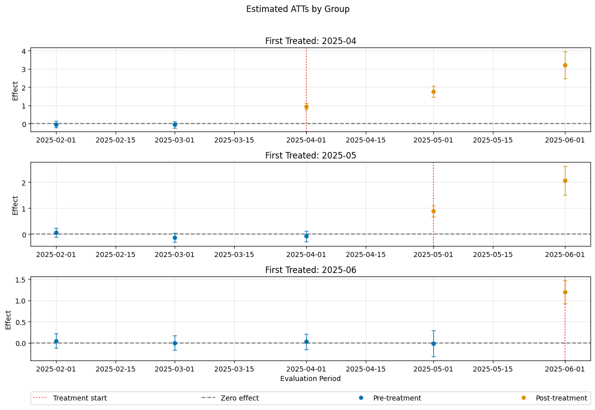
Linear Covariate Adjustment#
Remark that we relied on boosted trees to adjust for conditional parallel trends which allow for a nonlinear adjustment. In comparison to linear adjustment, we could rely on linear learners.
Remark that the DGP (``dgp_type=4``) is based on nonlinear conditional expectations such that the estimates will be biased
[17]:
linear_learners = {
    "ml_g": LinearRegression(),
    "ml_m": LogisticRegression(),
}

dml_obj_linear = DoubleMLDIDMulti(dml_data, **(default_args | linear_learners))
dml_obj_linear.fit()
dml_obj_linear.bootstrap(n_rep_boot=5000)
dml_obj_linear.plot_effects()
[17]:
(<Figure size 1200x800 with 4 Axes>,
 [<Axes: title={'center': 'First Treated: 2025-04'}, ylabel='Effect'>,
  <Axes: title={'center': 'First Treated: 2025-05'}, ylabel='Effect'>,
  <Axes: title={'center': 'First Treated: 2025-06'}, xlabel='Evaluation Period', ylabel='Effect'>])
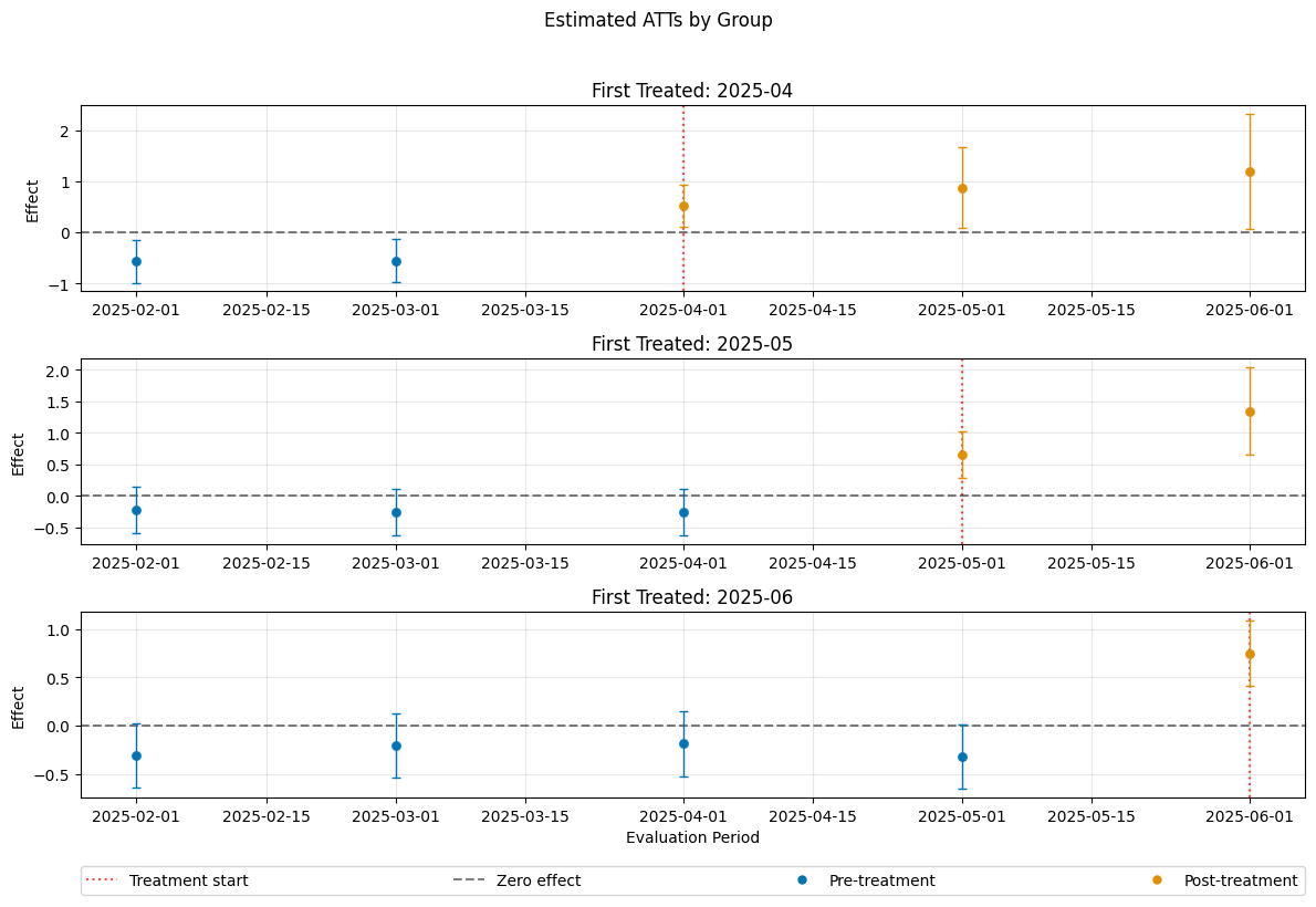
Aggregated Effects#
As the did-R-package, the \(ATT\)’s can be aggregated to summarize multiple effects. For details on different aggregations and details on their interpretations see Callaway and Sant’Anna(2021).
The aggregations are implemented via the aggregate() method.
Group Aggregation#
To obtain group-specific effects one can would like to average \(ATT(\mathrm{g}, t_\text{eval})\) over \(t_\text{eval}\). As a sample oracle we will combine all ite’s based on group \(\mathrm{g}\).
[18]:
df_post_treatment = df[df["t"] >= df["d"]]
df_post_treatment.groupby("d")["ite"].mean()
[18]:
d
2025-04-01    1.946796
2025-05-01    1.430767
2025-06-01    0.921234
Name: ite, dtype: float64
To obtain group-specific effects it is possible to aggregate several \(\widehat{ATT}(\mathrm{g},t_\text{pre},t_\text{eval})\) values based on the group \(\mathrm{g}\) by setting the aggregation="group" argument.
[19]:
aggregated_group = dml_obj.aggregate(aggregation="group")
print(aggregated_group)
_ = aggregated_group.plot_effects()
================== DoubleMLDIDAggregation Object ==================
 Group Aggregation

------------------ Overall Aggregated Effects ------------------
   coef  std err         t  P>|t|    2.5 %  97.5 %
1.36412 0.099185 13.753231    0.0 1.169721 1.55852
------------------ Aggregated Effects         ------------------
             coef   std err          t  P>|t|     2.5 %    97.5 %
2025-04  1.723058  0.169792  10.148059    0.0  1.390272  2.055844
2025-05  1.387994  0.117644  11.798250    0.0  1.157416  1.618573
2025-06  0.942530  0.092550  10.184013    0.0  0.761135  1.123924
------------------ Additional Information     ------------------
Score function: observational
Control group: never_treated
Anticipation periods: 0
/home/runner/work/doubleml-docs/doubleml-docs/doubleml-for-py/doubleml/did/did_aggregation.py:368: UserWarning: Joint confidence intervals require bootstrapping which hasn't been performed yet. Automatically applying '.aggregated_frameworks.bootstrap(method="normal", n_rep_boot=500)' with default values. For different bootstrap settings, call bootstrap() explicitly before plotting.
  warnings.warn(
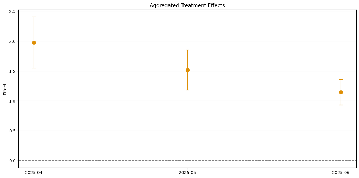
The output is a DoubleMLDIDAggregation object which includes an overall aggregation summary based on group size.
Time Aggregation#
To obtain time-specific effects one can would like to average \(ATT(\mathrm{g}, t_\text{eval})\) over \(\mathrm{g}\) (respecting group size). As a sample oracle we will combine all ite’s based on group \(\mathrm{g}\). As oracle values, we obtain
[20]:
df_post_treatment.groupby("t")["ite"].mean()
[20]:
t
2025-04-01    1.001738
2025-05-01    1.429849
2025-06-01    1.978681
Name: ite, dtype: float64
To aggregate \(\widehat{ATT}(\mathrm{g},t_\text{pre},t_\text{eval})\), based on \(t_\text{eval}\), but weighted with respect to group size. Corresponds to Calendar Time Effects from the did-R-package.
For calendar time effects set aggregation="time".
[21]:
aggregated_time = dml_obj.aggregate("time")
print(aggregated_time)
fig, ax = aggregated_time.plot_effects()
================== DoubleMLDIDAggregation Object ==================
 Time Aggregation

------------------ Overall Aggregated Effects ------------------
    coef  std err        t  P>|t|   2.5 %   97.5 %
1.358198 0.111113 12.22354    0.0 1.14042 1.575976
------------------ Aggregated Effects         ------------------
             coef   std err          t         P>|t|     2.5 %    97.5 %
2025-04  0.894345  0.114178   7.832897  4.662937e-15  0.670560  1.118130
2025-05  1.414416  0.128938  10.969749  0.000000e+00  1.161703  1.667130
2025-06  1.765831  0.137386  12.853107  0.000000e+00  1.496561  2.035102
------------------ Additional Information     ------------------
Score function: observational
Control group: never_treated
Anticipation periods: 0
/home/runner/work/doubleml-docs/doubleml-docs/doubleml-for-py/doubleml/did/did_aggregation.py:368: UserWarning: Joint confidence intervals require bootstrapping which hasn't been performed yet. Automatically applying '.aggregated_frameworks.bootstrap(method="normal", n_rep_boot=500)' with default values. For different bootstrap settings, call bootstrap() explicitly before plotting.
  warnings.warn(
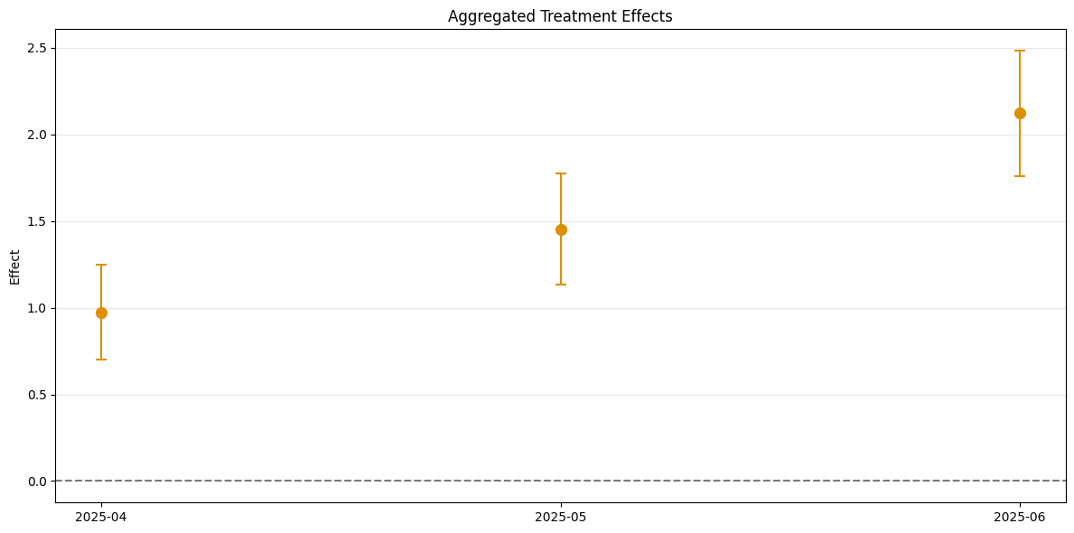
Event Study Aggregation#
To obtain event-study-type effects one can would like to aggregate \(ATT(\mathrm{g}, t_\text{eval})\) over \(e = t_\text{eval} - \mathrm{g}\) (respecting group size). As a sample oracle we will combine all ite’s based on group \(\mathrm{g}\). As oracle values, we obtain
[22]:
df["e"] = pd.to_datetime(df["t"]).values.astype("datetime64[M]") - \
    pd.to_datetime(df["d"]).values.astype("datetime64[M]")
df.groupby("e")["ite"].mean()[1:]
[22]:
e
-122 days   -0.052563
-92 days    -0.012523
-61 days     0.034187
-31 days     0.033022
0 days       0.940619
31 days      1.933388
59 days      2.938030
Name: ite, dtype: float64
Analogously, aggregation="eventstudy" aggregates \(\widehat{ATT}(\mathrm{g},t_\text{pre},t_\text{eval})\) based on exposure time \(e = t_\text{eval} - \mathrm{g}\) (respecting group size).
[23]:
aggregated_eventstudy = dml_obj.aggregate("eventstudy")
print(aggregated_eventstudy)
aggregated_eventstudy.plot_effects()
================== DoubleMLDIDAggregation Object ==================
 Event Study Aggregation

------------------ Overall Aggregated Effects ------------------
    coef  std err         t  P>|t|    2.5 %   97.5 %
1.737441 0.145784 11.917909    0.0 1.451709 2.023172
------------------ Aggregated Effects         ------------------
               coef   std err          t     P>|t|     2.5 %    97.5 %
-4 months  0.033767  0.085813   0.393492  0.693956 -0.134424  0.201957
-3 months -0.080302  0.070266  -1.142829  0.253109 -0.218020  0.057416
-2 months -0.070162  0.069257  -1.013059  0.311032 -0.205904  0.065580
-1 months -0.075756  0.070384  -1.076317  0.281786 -0.213707  0.062195
0 months   0.936289  0.068778  13.613176  0.000000  0.801487  1.071092
1 months   1.796715  0.151260  11.878349  0.000000  1.500251  2.093178
2 months   2.479317  0.254016   9.760474  0.000000  1.981455  2.977180
------------------ Additional Information     ------------------
Score function: observational
Control group: never_treated
Anticipation periods: 0
/home/runner/work/doubleml-docs/doubleml-docs/doubleml-for-py/doubleml/did/did_aggregation.py:368: UserWarning: Joint confidence intervals require bootstrapping which hasn't been performed yet. Automatically applying '.aggregated_frameworks.bootstrap(method="normal", n_rep_boot=500)' with default values. For different bootstrap settings, call bootstrap() explicitly before plotting.
  warnings.warn(
[23]:
(<Figure size 1200x600 with 1 Axes>,
 <Axes: title={'center': 'Aggregated Treatment Effects'}, ylabel='Effect'>)
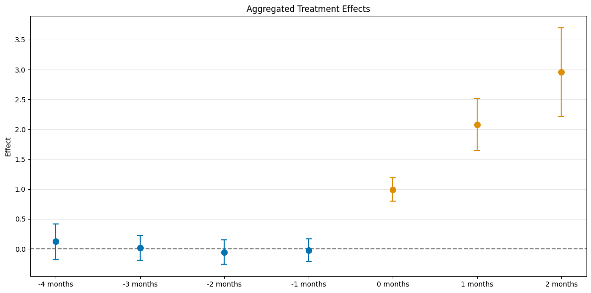
Aggregation Details#
The DoubleMLDIDAggregation objects include several DoubleMLFrameworks which support methods like bootstrap() or confint(). Further, the weights can be accessed via the properties
overall_aggregation_weights: weights for the overall aggregationaggregation_weights: weights for the aggregation
To clarify, e.g. for the eventstudy aggregation
[24]:
print(aggregated_eventstudy)
================== DoubleMLDIDAggregation Object ==================
 Event Study Aggregation

------------------ Overall Aggregated Effects ------------------
    coef  std err         t  P>|t|    2.5 %   97.5 %
1.737441 0.145784 11.917909    0.0 1.451709 2.023172
------------------ Aggregated Effects         ------------------
               coef   std err          t     P>|t|     2.5 %    97.5 %
-4 months  0.033767  0.085813   0.393492  0.693956 -0.134424  0.201957
-3 months -0.080302  0.070266  -1.142829  0.253109 -0.218020  0.057416
-2 months -0.070162  0.069257  -1.013059  0.311032 -0.205904  0.065580
-1 months -0.075756  0.070384  -1.076317  0.281786 -0.213707  0.062195
0 months   0.936289  0.068778  13.613176  0.000000  0.801487  1.071092
1 months   1.796715  0.151260  11.878349  0.000000  1.500251  2.093178
2 months   2.479317  0.254016   9.760474  0.000000  1.981455  2.977180
------------------ Additional Information     ------------------
Score function: observational
Control group: never_treated
Anticipation periods: 0
Here, the overall effect aggregation aggregates each effect with positive exposure
[25]:
print(aggregated_eventstudy.overall_aggregation_weights)
[0.         0.         0.         0.         0.33333333 0.33333333
 0.33333333]
If one would like to consider how the aggregated effect with \(e=0\) is computed, one would have to look at the corresponding set of weights within the aggregation_weights property
[26]:
# the weights for e=0 correspond to the fifth element of the aggregation weights
aggregated_eventstudy.aggregation_weights[4]
[26]:
array([0.        , 0.        , 0.36050921, 0.        , 0.        ,
       0.        , 0.        , 0.        , 0.31473456, 0.        ,
       0.        , 0.        , 0.        , 0.        , 0.32475623])
Taking a look at the original dml_obj, one can see that this combines the following estimates (only show month):
\(\widehat{ATT}(04,03,04)\)
\(\widehat{ATT}(05,04,05)\)
\(\widehat{ATT}(06,05,06)\)
[27]:
print(dml_obj.summary["coef"])
ATT(2025-04,2025-01,2025-02)   -0.077634
ATT(2025-04,2025-02,2025-03)   -0.120883
ATT(2025-04,2025-03,2025-04)    0.894345
ATT(2025-04,2025-03,2025-05)    1.795511
ATT(2025-04,2025-03,2025-06)    2.479317
ATT(2025-05,2025-01,2025-02)   -0.169782
ATT(2025-05,2025-02,2025-03)   -0.119620
ATT(2025-05,2025-03,2025-04)   -0.132521
ATT(2025-05,2025-04,2025-05)    0.977895
ATT(2025-05,2025-04,2025-06)    1.798093
ATT(2025-06,2025-01,2025-02)    0.033767
ATT(2025-06,2025-02,2025-03)    0.006418
ATT(2025-06,2025-03,2025-04)   -0.013935
ATT(2025-06,2025-04,2025-05)    0.029352
ATT(2025-06,2025-05,2025-06)    0.942530
Name: coef, dtype: float64
Anticipation#
As described in the Model Guide, one can include anticipation periods \(\delta>0\) by setting the anticipation_periods parameter.
Data with Anticipation#
The DGP allows to include anticipation periods via the anticipation_periods parameter. In this case the observations will be “shifted” such that units anticipate the effect earlier and the exposure effect is increased by the number of periods where the effect is anticipated.
[28]:
n_obs = 4000
n_periods = 6

df_anticipation = make_did_CS2021(n_obs, dgp_type=4, n_periods=n_periods, n_pre_treat_periods=3, time_type="datetime", anticipation_periods=1)

print(df_anticipation.shape)
df_anticipation.head()
(19410, 10)
[28]:
| id | y | y0 | y1 | d | t | Z1 | Z2 | Z3 | Z4 | |
|---|---|---|---|---|---|---|---|---|---|---|
| 1 | 0 | 208.594874 | 208.594874 | 208.231811 | 2025-06-01 | 2025-01-01 | -0.537974 | 0.869105 | 0.49675 | 0.811849 |
| 2 | 0 | 205.187155 | 205.187155 | 206.099880 | 2025-06-01 | 2025-02-01 | -0.537974 | 0.869105 | 0.49675 | 0.811849 |
| 3 | 0 | 206.228241 | 206.228241 | 207.902692 | 2025-06-01 | 2025-03-01 | -0.537974 | 0.869105 | 0.49675 | 0.811849 |
| 4 | 0 | 204.576914 | 204.576914 | 204.784454 | 2025-06-01 | 2025-04-01 | -0.537974 | 0.869105 | 0.49675 | 0.811849 |
| 5 | 0 | 205.033872 | 202.869407 | 205.033872 | 2025-06-01 | 2025-05-01 | -0.537974 | 0.869105 | 0.49675 | 0.811849 |
To visualize the anticipation, we will again plot the “oracle” values
[29]:
df_anticipation["ite"] = df_anticipation["y1"] - df_anticipation["y0"]
df_anticipation["First Treated"] = df_anticipation["d"].dt.strftime("%Y-%m").fillna("Never Treated")
agg_df_anticipation = df_anticipation.groupby(["t", "First Treated"]).agg(**agg_dictionary).reset_index()
agg_df_anticipation.head()
[29]:
| t | First Treated | y_mean | y_lower_quantile | y_upper_quantile | ite_mean | ite_lower_quantile | ite_upper_quantile | |
|---|---|---|---|---|---|---|---|---|
| 0 | 2025-01-01 | 2025-04 | 208.816145 | 190.889575 | 226.924235 | -0.008842 | -2.350612 | 2.392154 |
| 1 | 2025-01-01 | 2025-05 | 210.637015 | 194.640691 | 226.625596 | -0.033535 | -2.531033 | 2.361308 |
| 2 | 2025-01-01 | 2025-06 | 212.825793 | 195.664713 | 229.576897 | -0.013461 | -2.344146 | 2.482600 |
| 3 | 2025-01-01 | Never Treated | 217.704239 | 201.029963 | 235.911643 | -0.009008 | -2.389302 | 2.339801 |
| 4 | 2025-02-01 | 2025-04 | 208.850873 | 183.208505 | 234.510316 | -0.062110 | -2.392163 | 2.313700 |
One can see that the effect is already anticipated one period before the actual treatment assignment.
[30]:
plot_data(agg_df_anticipation, col_name='ite')
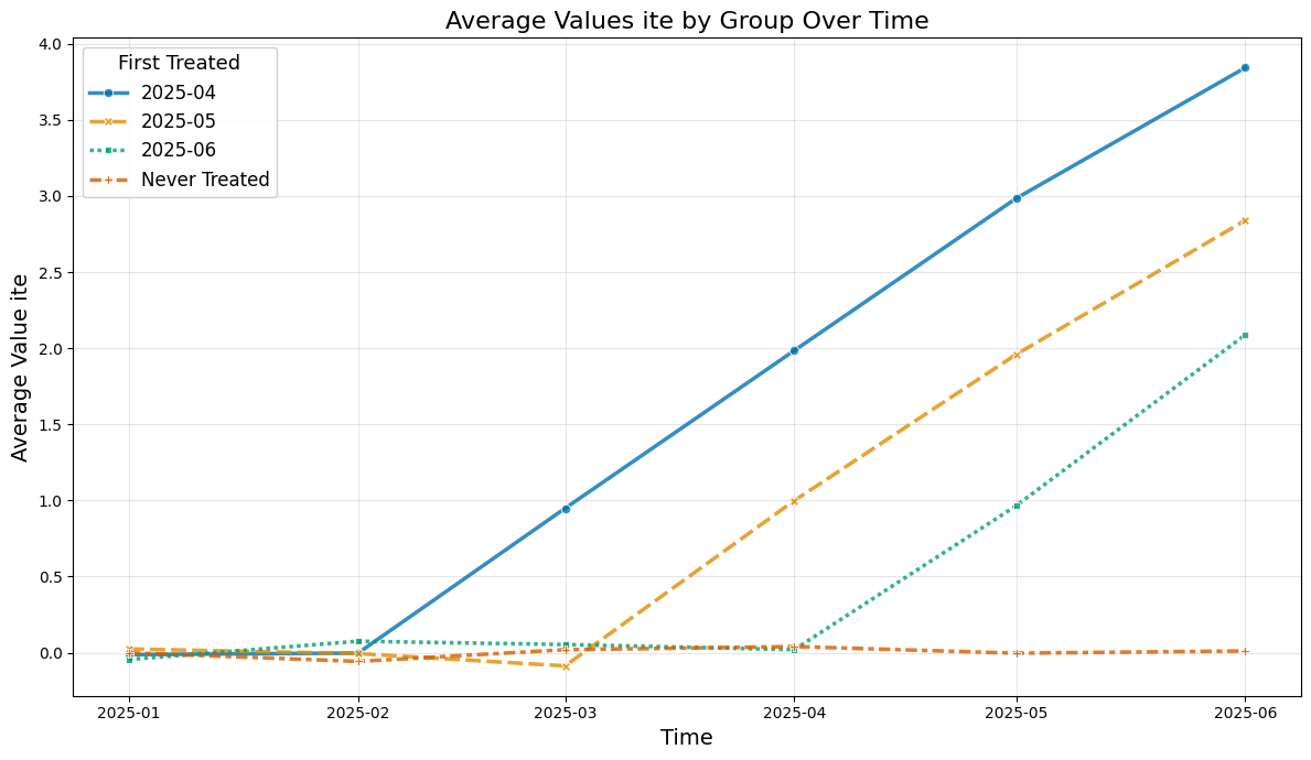
Initialize a corresponding DoubleMLPanelData object.
[31]:
dml_data_anticipation = DoubleMLPanelData(
    data=df_anticipation,
    y_col="y",
    d_cols="d",
    id_col="id",
    t_col="t",
    x_cols=["Z1", "Z2", "Z3", "Z4"],
    datetime_unit="M"
)
ATT Estimation#
Let us take a look at the estimation without anticipation.
[32]:
dml_obj_anticipation = DoubleMLDIDMulti(dml_data_anticipation, **default_args)
dml_obj_anticipation.fit()
dml_obj_anticipation.bootstrap(n_rep_boot=5000)
dml_obj_anticipation.plot_effects()
/opt/hostedtoolcache/Python/3.12.13/x64/lib/python3.12/site-packages/sklearn/utils/validation.py:2739: UserWarning: X does not have valid feature names, but LGBMRegressor was fitted with feature names
  warnings.warn(
/opt/hostedtoolcache/Python/3.12.13/x64/lib/python3.12/site-packages/sklearn/utils/validation.py:2739: UserWarning: X does not have valid feature names, but LGBMRegressor was fitted with feature names
  warnings.warn(
/opt/hostedtoolcache/Python/3.12.13/x64/lib/python3.12/site-packages/sklearn/utils/validation.py:2739: UserWarning: X does not have valid feature names, but LGBMRegressor was fitted with feature names
  warnings.warn(
/opt/hostedtoolcache/Python/3.12.13/x64/lib/python3.12/site-packages/sklearn/utils/validation.py:2739: UserWarning: X does not have valid feature names, but LGBMRegressor was fitted with feature names
  warnings.warn(
/opt/hostedtoolcache/Python/3.12.13/x64/lib/python3.12/site-packages/sklearn/utils/validation.py:2739: UserWarning: X does not have valid feature names, but LGBMRegressor was fitted with feature names
  warnings.warn(
/opt/hostedtoolcache/Python/3.12.13/x64/lib/python3.12/site-packages/sklearn/utils/validation.py:2739: UserWarning: X does not have valid feature names, but LGBMRegressor was fitted with feature names
  warnings.warn(
/opt/hostedtoolcache/Python/3.12.13/x64/lib/python3.12/site-packages/sklearn/utils/validation.py:2739: UserWarning: X does not have valid feature names, but LGBMRegressor was fitted with feature names
  warnings.warn(
/opt/hostedtoolcache/Python/3.12.13/x64/lib/python3.12/site-packages/sklearn/utils/validation.py:2739: UserWarning: X does not have valid feature names, but LGBMRegressor was fitted with feature names
  warnings.warn(
/opt/hostedtoolcache/Python/3.12.13/x64/lib/python3.12/site-packages/sklearn/utils/validation.py:2739: UserWarning: X does not have valid feature names, but LGBMRegressor was fitted with feature names
  warnings.warn(
/opt/hostedtoolcache/Python/3.12.13/x64/lib/python3.12/site-packages/sklearn/utils/validation.py:2739: UserWarning: X does not have valid feature names, but LGBMRegressor was fitted with feature names
  warnings.warn(
/opt/hostedtoolcache/Python/3.12.13/x64/lib/python3.12/site-packages/sklearn/utils/validation.py:2739: UserWarning: X does not have valid feature names, but LGBMClassifier was fitted with feature names
  warnings.warn(
/opt/hostedtoolcache/Python/3.12.13/x64/lib/python3.12/site-packages/sklearn/utils/validation.py:2739: UserWarning: X does not have valid feature names, but LGBMClassifier was fitted with feature names
  warnings.warn(
/opt/hostedtoolcache/Python/3.12.13/x64/lib/python3.12/site-packages/sklearn/utils/validation.py:2739: UserWarning: X does not have valid feature names, but LGBMClassifier was fitted with feature names
  warnings.warn(
/opt/hostedtoolcache/Python/3.12.13/x64/lib/python3.12/site-packages/sklearn/utils/validation.py:2739: UserWarning: X does not have valid feature names, but LGBMClassifier was fitted with feature names
  warnings.warn(
/opt/hostedtoolcache/Python/3.12.13/x64/lib/python3.12/site-packages/sklearn/utils/validation.py:2739: UserWarning: X does not have valid feature names, but LGBMClassifier was fitted with feature names
  warnings.warn(
/opt/hostedtoolcache/Python/3.12.13/x64/lib/python3.12/site-packages/sklearn/utils/validation.py:2739: UserWarning: X does not have valid feature names, but LGBMRegressor was fitted with feature names
  warnings.warn(
/opt/hostedtoolcache/Python/3.12.13/x64/lib/python3.12/site-packages/sklearn/utils/validation.py:2739: UserWarning: X does not have valid feature names, but LGBMRegressor was fitted with feature names
  warnings.warn(
/opt/hostedtoolcache/Python/3.12.13/x64/lib/python3.12/site-packages/sklearn/utils/validation.py:2739: UserWarning: X does not have valid feature names, but LGBMRegressor was fitted with feature names
  warnings.warn(
/opt/hostedtoolcache/Python/3.12.13/x64/lib/python3.12/site-packages/sklearn/utils/validation.py:2739: UserWarning: X does not have valid feature names, but LGBMRegressor was fitted with feature names
  warnings.warn(
/opt/hostedtoolcache/Python/3.12.13/x64/lib/python3.12/site-packages/sklearn/utils/validation.py:2739: UserWarning: X does not have valid feature names, but LGBMRegressor was fitted with feature names
  warnings.warn(
/opt/hostedtoolcache/Python/3.12.13/x64/lib/python3.12/site-packages/sklearn/utils/validation.py:2739: UserWarning: X does not have valid feature names, but LGBMRegressor was fitted with feature names
  warnings.warn(
/opt/hostedtoolcache/Python/3.12.13/x64/lib/python3.12/site-packages/sklearn/utils/validation.py:2739: UserWarning: X does not have valid feature names, but LGBMRegressor was fitted with feature names
  warnings.warn(
/opt/hostedtoolcache/Python/3.12.13/x64/lib/python3.12/site-packages/sklearn/utils/validation.py:2739: UserWarning: X does not have valid feature names, but LGBMRegressor was fitted with feature names
  warnings.warn(
/opt/hostedtoolcache/Python/3.12.13/x64/lib/python3.12/site-packages/sklearn/utils/validation.py:2739: UserWarning: X does not have valid feature names, but LGBMRegressor was fitted with feature names
  warnings.warn(
/opt/hostedtoolcache/Python/3.12.13/x64/lib/python3.12/site-packages/sklearn/utils/validation.py:2739: UserWarning: X does not have valid feature names, but LGBMRegressor was fitted with feature names
  warnings.warn(
/opt/hostedtoolcache/Python/3.12.13/x64/lib/python3.12/site-packages/sklearn/utils/validation.py:2739: UserWarning: X does not have valid feature names, but LGBMClassifier was fitted with feature names
  warnings.warn(
/opt/hostedtoolcache/Python/3.12.13/x64/lib/python3.12/site-packages/sklearn/utils/validation.py:2739: UserWarning: X does not have valid feature names, but LGBMClassifier was fitted with feature names
  warnings.warn(
/opt/hostedtoolcache/Python/3.12.13/x64/lib/python3.12/site-packages/sklearn/utils/validation.py:2739: UserWarning: X does not have valid feature names, but LGBMClassifier was fitted with feature names
  warnings.warn(
/opt/hostedtoolcache/Python/3.12.13/x64/lib/python3.12/site-packages/sklearn/utils/validation.py:2739: UserWarning: X does not have valid feature names, but LGBMClassifier was fitted with feature names
  warnings.warn(
/opt/hostedtoolcache/Python/3.12.13/x64/lib/python3.12/site-packages/sklearn/utils/validation.py:2739: UserWarning: X does not have valid feature names, but LGBMClassifier was fitted with feature names
  warnings.warn(
/opt/hostedtoolcache/Python/3.12.13/x64/lib/python3.12/site-packages/sklearn/utils/validation.py:2739: UserWarning: X does not have valid feature names, but LGBMRegressor was fitted with feature names
  warnings.warn(
/opt/hostedtoolcache/Python/3.12.13/x64/lib/python3.12/site-packages/sklearn/utils/validation.py:2739: UserWarning: X does not have valid feature names, but LGBMRegressor was fitted with feature names
  warnings.warn(
/opt/hostedtoolcache/Python/3.12.13/x64/lib/python3.12/site-packages/sklearn/utils/validation.py:2739: UserWarning: X does not have valid feature names, but LGBMRegressor was fitted with feature names
  warnings.warn(
/opt/hostedtoolcache/Python/3.12.13/x64/lib/python3.12/site-packages/sklearn/utils/validation.py:2739: UserWarning: X does not have valid feature names, but LGBMRegressor was fitted with feature names
  warnings.warn(
/opt/hostedtoolcache/Python/3.12.13/x64/lib/python3.12/site-packages/sklearn/utils/validation.py:2739: UserWarning: X does not have valid feature names, but LGBMRegressor was fitted with feature names
  warnings.warn(
/opt/hostedtoolcache/Python/3.12.13/x64/lib/python3.12/site-packages/sklearn/utils/validation.py:2739: UserWarning: X does not have valid feature names, but LGBMRegressor was fitted with feature names
  warnings.warn(
/opt/hostedtoolcache/Python/3.12.13/x64/lib/python3.12/site-packages/sklearn/utils/validation.py:2739: UserWarning: X does not have valid feature names, but LGBMRegressor was fitted with feature names
  warnings.warn(
/opt/hostedtoolcache/Python/3.12.13/x64/lib/python3.12/site-packages/sklearn/utils/validation.py:2739: UserWarning: X does not have valid feature names, but LGBMRegressor was fitted with feature names
  warnings.warn(
/opt/hostedtoolcache/Python/3.12.13/x64/lib/python3.12/site-packages/sklearn/utils/validation.py:2739: UserWarning: X does not have valid feature names, but LGBMRegressor was fitted with feature names
  warnings.warn(
/opt/hostedtoolcache/Python/3.12.13/x64/lib/python3.12/site-packages/sklearn/utils/validation.py:2739: UserWarning: X does not have valid feature names, but LGBMRegressor was fitted with feature names
  warnings.warn(
/opt/hostedtoolcache/Python/3.12.13/x64/lib/python3.12/site-packages/sklearn/utils/validation.py:2739: UserWarning: X does not have valid feature names, but LGBMClassifier was fitted with feature names
  warnings.warn(
/opt/hostedtoolcache/Python/3.12.13/x64/lib/python3.12/site-packages/sklearn/utils/validation.py:2739: UserWarning: X does not have valid feature names, but LGBMClassifier was fitted with feature names
  warnings.warn(
/opt/hostedtoolcache/Python/3.12.13/x64/lib/python3.12/site-packages/sklearn/utils/validation.py:2739: UserWarning: X does not have valid feature names, but LGBMClassifier was fitted with feature names
  warnings.warn(
/opt/hostedtoolcache/Python/3.12.13/x64/lib/python3.12/site-packages/sklearn/utils/validation.py:2739: UserWarning: X does not have valid feature names, but LGBMClassifier was fitted with feature names
  warnings.warn(
/opt/hostedtoolcache/Python/3.12.13/x64/lib/python3.12/site-packages/sklearn/utils/validation.py:2739: UserWarning: X does not have valid feature names, but LGBMClassifier was fitted with feature names
  warnings.warn(
/opt/hostedtoolcache/Python/3.12.13/x64/lib/python3.12/site-packages/sklearn/utils/validation.py:2739: UserWarning: X does not have valid feature names, but LGBMRegressor was fitted with feature names
  warnings.warn(
/opt/hostedtoolcache/Python/3.12.13/x64/lib/python3.12/site-packages/sklearn/utils/validation.py:2739: UserWarning: X does not have valid feature names, but LGBMRegressor was fitted with feature names
  warnings.warn(
/opt/hostedtoolcache/Python/3.12.13/x64/lib/python3.12/site-packages/sklearn/utils/validation.py:2739: UserWarning: X does not have valid feature names, but LGBMRegressor was fitted with feature names
  warnings.warn(
/opt/hostedtoolcache/Python/3.12.13/x64/lib/python3.12/site-packages/sklearn/utils/validation.py:2739: UserWarning: X does not have valid feature names, but LGBMRegressor was fitted with feature names
  warnings.warn(
/opt/hostedtoolcache/Python/3.12.13/x64/lib/python3.12/site-packages/sklearn/utils/validation.py:2739: UserWarning: X does not have valid feature names, but LGBMRegressor was fitted with feature names
  warnings.warn(
/opt/hostedtoolcache/Python/3.12.13/x64/lib/python3.12/site-packages/sklearn/utils/validation.py:2739: UserWarning: X does not have valid feature names, but LGBMRegressor was fitted with feature names
  warnings.warn(
/opt/hostedtoolcache/Python/3.12.13/x64/lib/python3.12/site-packages/sklearn/utils/validation.py:2739: UserWarning: X does not have valid feature names, but LGBMRegressor was fitted with feature names
  warnings.warn(
/opt/hostedtoolcache/Python/3.12.13/x64/lib/python3.12/site-packages/sklearn/utils/validation.py:2739: UserWarning: X does not have valid feature names, but LGBMRegressor was fitted with feature names
  warnings.warn(
/opt/hostedtoolcache/Python/3.12.13/x64/lib/python3.12/site-packages/sklearn/utils/validation.py:2739: UserWarning: X does not have valid feature names, but LGBMRegressor was fitted with feature names
  warnings.warn(
/opt/hostedtoolcache/Python/3.12.13/x64/lib/python3.12/site-packages/sklearn/utils/validation.py:2739: UserWarning: X does not have valid feature names, but LGBMRegressor was fitted with feature names
  warnings.warn(
/opt/hostedtoolcache/Python/3.12.13/x64/lib/python3.12/site-packages/sklearn/utils/validation.py:2739: UserWarning: X does not have valid feature names, but LGBMClassifier was fitted with feature names
  warnings.warn(
/opt/hostedtoolcache/Python/3.12.13/x64/lib/python3.12/site-packages/sklearn/utils/validation.py:2739: UserWarning: X does not have valid feature names, but LGBMClassifier was fitted with feature names
  warnings.warn(
/opt/hostedtoolcache/Python/3.12.13/x64/lib/python3.12/site-packages/sklearn/utils/validation.py:2739: UserWarning: X does not have valid feature names, but LGBMClassifier was fitted with feature names
  warnings.warn(
/opt/hostedtoolcache/Python/3.12.13/x64/lib/python3.12/site-packages/sklearn/utils/validation.py:2739: UserWarning: X does not have valid feature names, but LGBMClassifier was fitted with feature names
  warnings.warn(
/opt/hostedtoolcache/Python/3.12.13/x64/lib/python3.12/site-packages/sklearn/utils/validation.py:2739: UserWarning: X does not have valid feature names, but LGBMClassifier was fitted with feature names
  warnings.warn(
/opt/hostedtoolcache/Python/3.12.13/x64/lib/python3.12/site-packages/sklearn/utils/validation.py:2739: UserWarning: X does not have valid feature names, but LGBMRegressor was fitted with feature names
  warnings.warn(
/opt/hostedtoolcache/Python/3.12.13/x64/lib/python3.12/site-packages/sklearn/utils/validation.py:2739: UserWarning: X does not have valid feature names, but LGBMRegressor was fitted with feature names
  warnings.warn(
/opt/hostedtoolcache/Python/3.12.13/x64/lib/python3.12/site-packages/sklearn/utils/validation.py:2739: UserWarning: X does not have valid feature names, but LGBMRegressor was fitted with feature names
  warnings.warn(
/opt/hostedtoolcache/Python/3.12.13/x64/lib/python3.12/site-packages/sklearn/utils/validation.py:2739: UserWarning: X does not have valid feature names, but LGBMRegressor was fitted with feature names
  warnings.warn(
/opt/hostedtoolcache/Python/3.12.13/x64/lib/python3.12/site-packages/sklearn/utils/validation.py:2739: UserWarning: X does not have valid feature names, but LGBMRegressor was fitted with feature names
  warnings.warn(
/opt/hostedtoolcache/Python/3.12.13/x64/lib/python3.12/site-packages/sklearn/utils/validation.py:2739: UserWarning: X does not have valid feature names, but LGBMRegressor was fitted with feature names
  warnings.warn(
/opt/hostedtoolcache/Python/3.12.13/x64/lib/python3.12/site-packages/sklearn/utils/validation.py:2739: UserWarning: X does not have valid feature names, but LGBMRegressor was fitted with feature names
  warnings.warn(
/opt/hostedtoolcache/Python/3.12.13/x64/lib/python3.12/site-packages/sklearn/utils/validation.py:2739: UserWarning: X does not have valid feature names, but LGBMRegressor was fitted with feature names
  warnings.warn(
/opt/hostedtoolcache/Python/3.12.13/x64/lib/python3.12/site-packages/sklearn/utils/validation.py:2739: UserWarning: X does not have valid feature names, but LGBMRegressor was fitted with feature names
  warnings.warn(
/opt/hostedtoolcache/Python/3.12.13/x64/lib/python3.12/site-packages/sklearn/utils/validation.py:2739: UserWarning: X does not have valid feature names, but LGBMRegressor was fitted with feature names
  warnings.warn(
/opt/hostedtoolcache/Python/3.12.13/x64/lib/python3.12/site-packages/sklearn/utils/validation.py:2739: UserWarning: X does not have valid feature names, but LGBMClassifier was fitted with feature names
  warnings.warn(
/opt/hostedtoolcache/Python/3.12.13/x64/lib/python3.12/site-packages/sklearn/utils/validation.py:2739: UserWarning: X does not have valid feature names, but LGBMClassifier was fitted with feature names
  warnings.warn(
/opt/hostedtoolcache/Python/3.12.13/x64/lib/python3.12/site-packages/sklearn/utils/validation.py:2739: UserWarning: X does not have valid feature names, but LGBMClassifier was fitted with feature names
  warnings.warn(
/opt/hostedtoolcache/Python/3.12.13/x64/lib/python3.12/site-packages/sklearn/utils/validation.py:2739: UserWarning: X does not have valid feature names, but LGBMClassifier was fitted with feature names
  warnings.warn(
/opt/hostedtoolcache/Python/3.12.13/x64/lib/python3.12/site-packages/sklearn/utils/validation.py:2739: UserWarning: X does not have valid feature names, but LGBMClassifier was fitted with feature names
  warnings.warn(
/opt/hostedtoolcache/Python/3.12.13/x64/lib/python3.12/site-packages/sklearn/utils/validation.py:2739: UserWarning: X does not have valid feature names, but LGBMRegressor was fitted with feature names
  warnings.warn(
/opt/hostedtoolcache/Python/3.12.13/x64/lib/python3.12/site-packages/sklearn/utils/validation.py:2739: UserWarning: X does not have valid feature names, but LGBMRegressor was fitted with feature names
  warnings.warn(
/opt/hostedtoolcache/Python/3.12.13/x64/lib/python3.12/site-packages/sklearn/utils/validation.py:2739: UserWarning: X does not have valid feature names, but LGBMRegressor was fitted with feature names
  warnings.warn(
/opt/hostedtoolcache/Python/3.12.13/x64/lib/python3.12/site-packages/sklearn/utils/validation.py:2739: UserWarning: X does not have valid feature names, but LGBMRegressor was fitted with feature names
  warnings.warn(
/opt/hostedtoolcache/Python/3.12.13/x64/lib/python3.12/site-packages/sklearn/utils/validation.py:2739: UserWarning: X does not have valid feature names, but LGBMRegressor was fitted with feature names
  warnings.warn(
/opt/hostedtoolcache/Python/3.12.13/x64/lib/python3.12/site-packages/sklearn/utils/validation.py:2739: UserWarning: X does not have valid feature names, but LGBMRegressor was fitted with feature names
  warnings.warn(
/opt/hostedtoolcache/Python/3.12.13/x64/lib/python3.12/site-packages/sklearn/utils/validation.py:2739: UserWarning: X does not have valid feature names, but LGBMRegressor was fitted with feature names
  warnings.warn(
/opt/hostedtoolcache/Python/3.12.13/x64/lib/python3.12/site-packages/sklearn/utils/validation.py:2739: UserWarning: X does not have valid feature names, but LGBMRegressor was fitted with feature names
  warnings.warn(
/opt/hostedtoolcache/Python/3.12.13/x64/lib/python3.12/site-packages/sklearn/utils/validation.py:2739: UserWarning: X does not have valid feature names, but LGBMRegressor was fitted with feature names
  warnings.warn(
/opt/hostedtoolcache/Python/3.12.13/x64/lib/python3.12/site-packages/sklearn/utils/validation.py:2739: UserWarning: X does not have valid feature names, but LGBMRegressor was fitted with feature names
  warnings.warn(
/opt/hostedtoolcache/Python/3.12.13/x64/lib/python3.12/site-packages/sklearn/utils/validation.py:2739: UserWarning: X does not have valid feature names, but LGBMClassifier was fitted with feature names
  warnings.warn(
/opt/hostedtoolcache/Python/3.12.13/x64/lib/python3.12/site-packages/sklearn/utils/validation.py:2739: UserWarning: X does not have valid feature names, but LGBMClassifier was fitted with feature names
  warnings.warn(
/opt/hostedtoolcache/Python/3.12.13/x64/lib/python3.12/site-packages/sklearn/utils/validation.py:2739: UserWarning: X does not have valid feature names, but LGBMClassifier was fitted with feature names
  warnings.warn(
/opt/hostedtoolcache/Python/3.12.13/x64/lib/python3.12/site-packages/sklearn/utils/validation.py:2739: UserWarning: X does not have valid feature names, but LGBMClassifier was fitted with feature names
  warnings.warn(
/opt/hostedtoolcache/Python/3.12.13/x64/lib/python3.12/site-packages/sklearn/utils/validation.py:2739: UserWarning: X does not have valid feature names, but LGBMClassifier was fitted with feature names
  warnings.warn(
/opt/hostedtoolcache/Python/3.12.13/x64/lib/python3.12/site-packages/sklearn/utils/validation.py:2739: UserWarning: X does not have valid feature names, but LGBMRegressor was fitted with feature names
  warnings.warn(
/opt/hostedtoolcache/Python/3.12.13/x64/lib/python3.12/site-packages/sklearn/utils/validation.py:2739: UserWarning: X does not have valid feature names, but LGBMRegressor was fitted with feature names
  warnings.warn(
/opt/hostedtoolcache/Python/3.12.13/x64/lib/python3.12/site-packages/sklearn/utils/validation.py:2739: UserWarning: X does not have valid feature names, but LGBMRegressor was fitted with feature names
  warnings.warn(
/opt/hostedtoolcache/Python/3.12.13/x64/lib/python3.12/site-packages/sklearn/utils/validation.py:2739: UserWarning: X does not have valid feature names, but LGBMRegressor was fitted with feature names
  warnings.warn(
/opt/hostedtoolcache/Python/3.12.13/x64/lib/python3.12/site-packages/sklearn/utils/validation.py:2739: UserWarning: X does not have valid feature names, but LGBMRegressor was fitted with feature names
  warnings.warn(
/opt/hostedtoolcache/Python/3.12.13/x64/lib/python3.12/site-packages/sklearn/utils/validation.py:2739: UserWarning: X does not have valid feature names, but LGBMRegressor was fitted with feature names
  warnings.warn(
/opt/hostedtoolcache/Python/3.12.13/x64/lib/python3.12/site-packages/sklearn/utils/validation.py:2739: UserWarning: X does not have valid feature names, but LGBMRegressor was fitted with feature names
  warnings.warn(
/opt/hostedtoolcache/Python/3.12.13/x64/lib/python3.12/site-packages/sklearn/utils/validation.py:2739: UserWarning: X does not have valid feature names, but LGBMRegressor was fitted with feature names
  warnings.warn(
/opt/hostedtoolcache/Python/3.12.13/x64/lib/python3.12/site-packages/sklearn/utils/validation.py:2739: UserWarning: X does not have valid feature names, but LGBMRegressor was fitted with feature names
  warnings.warn(
/opt/hostedtoolcache/Python/3.12.13/x64/lib/python3.12/site-packages/sklearn/utils/validation.py:2739: UserWarning: X does not have valid feature names, but LGBMRegressor was fitted with feature names
  warnings.warn(
/opt/hostedtoolcache/Python/3.12.13/x64/lib/python3.12/site-packages/sklearn/utils/validation.py:2739: UserWarning: X does not have valid feature names, but LGBMClassifier was fitted with feature names
  warnings.warn(
/opt/hostedtoolcache/Python/3.12.13/x64/lib/python3.12/site-packages/sklearn/utils/validation.py:2739: UserWarning: X does not have valid feature names, but LGBMClassifier was fitted with feature names
  warnings.warn(
/opt/hostedtoolcache/Python/3.12.13/x64/lib/python3.12/site-packages/sklearn/utils/validation.py:2739: UserWarning: X does not have valid feature names, but LGBMClassifier was fitted with feature names
  warnings.warn(
/opt/hostedtoolcache/Python/3.12.13/x64/lib/python3.12/site-packages/sklearn/utils/validation.py:2739: UserWarning: X does not have valid feature names, but LGBMClassifier was fitted with feature names
  warnings.warn(
/opt/hostedtoolcache/Python/3.12.13/x64/lib/python3.12/site-packages/sklearn/utils/validation.py:2739: UserWarning: X does not have valid feature names, but LGBMClassifier was fitted with feature names
  warnings.warn(
/opt/hostedtoolcache/Python/3.12.13/x64/lib/python3.12/site-packages/sklearn/utils/validation.py:2739: UserWarning: X does not have valid feature names, but LGBMRegressor was fitted with feature names
  warnings.warn(
/opt/hostedtoolcache/Python/3.12.13/x64/lib/python3.12/site-packages/sklearn/utils/validation.py:2739: UserWarning: X does not have valid feature names, but LGBMRegressor was fitted with feature names
  warnings.warn(
/opt/hostedtoolcache/Python/3.12.13/x64/lib/python3.12/site-packages/sklearn/utils/validation.py:2739: UserWarning: X does not have valid feature names, but LGBMRegressor was fitted with feature names
  warnings.warn(
/opt/hostedtoolcache/Python/3.12.13/x64/lib/python3.12/site-packages/sklearn/utils/validation.py:2739: UserWarning: X does not have valid feature names, but LGBMRegressor was fitted with feature names
  warnings.warn(
/opt/hostedtoolcache/Python/3.12.13/x64/lib/python3.12/site-packages/sklearn/utils/validation.py:2739: UserWarning: X does not have valid feature names, but LGBMRegressor was fitted with feature names
  warnings.warn(
/opt/hostedtoolcache/Python/3.12.13/x64/lib/python3.12/site-packages/sklearn/utils/validation.py:2739: UserWarning: X does not have valid feature names, but LGBMRegressor was fitted with feature names
  warnings.warn(
/opt/hostedtoolcache/Python/3.12.13/x64/lib/python3.12/site-packages/sklearn/utils/validation.py:2739: UserWarning: X does not have valid feature names, but LGBMRegressor was fitted with feature names
  warnings.warn(
/opt/hostedtoolcache/Python/3.12.13/x64/lib/python3.12/site-packages/sklearn/utils/validation.py:2739: UserWarning: X does not have valid feature names, but LGBMRegressor was fitted with feature names
  warnings.warn(
/opt/hostedtoolcache/Python/3.12.13/x64/lib/python3.12/site-packages/sklearn/utils/validation.py:2739: UserWarning: X does not have valid feature names, but LGBMRegressor was fitted with feature names
  warnings.warn(
/opt/hostedtoolcache/Python/3.12.13/x64/lib/python3.12/site-packages/sklearn/utils/validation.py:2739: UserWarning: X does not have valid feature names, but LGBMRegressor was fitted with feature names
  warnings.warn(
/opt/hostedtoolcache/Python/3.12.13/x64/lib/python3.12/site-packages/sklearn/utils/validation.py:2739: UserWarning: X does not have valid feature names, but LGBMClassifier was fitted with feature names
  warnings.warn(
/opt/hostedtoolcache/Python/3.12.13/x64/lib/python3.12/site-packages/sklearn/utils/validation.py:2739: UserWarning: X does not have valid feature names, but LGBMClassifier was fitted with feature names
  warnings.warn(
/opt/hostedtoolcache/Python/3.12.13/x64/lib/python3.12/site-packages/sklearn/utils/validation.py:2739: UserWarning: X does not have valid feature names, but LGBMClassifier was fitted with feature names
  warnings.warn(
/opt/hostedtoolcache/Python/3.12.13/x64/lib/python3.12/site-packages/sklearn/utils/validation.py:2739: UserWarning: X does not have valid feature names, but LGBMClassifier was fitted with feature names
  warnings.warn(
/opt/hostedtoolcache/Python/3.12.13/x64/lib/python3.12/site-packages/sklearn/utils/validation.py:2739: UserWarning: X does not have valid feature names, but LGBMClassifier was fitted with feature names
  warnings.warn(
/opt/hostedtoolcache/Python/3.12.13/x64/lib/python3.12/site-packages/sklearn/utils/validation.py:2739: UserWarning: X does not have valid feature names, but LGBMRegressor was fitted with feature names
  warnings.warn(
/opt/hostedtoolcache/Python/3.12.13/x64/lib/python3.12/site-packages/sklearn/utils/validation.py:2739: UserWarning: X does not have valid feature names, but LGBMRegressor was fitted with feature names
  warnings.warn(
/opt/hostedtoolcache/Python/3.12.13/x64/lib/python3.12/site-packages/sklearn/utils/validation.py:2739: UserWarning: X does not have valid feature names, but LGBMRegressor was fitted with feature names
  warnings.warn(
/opt/hostedtoolcache/Python/3.12.13/x64/lib/python3.12/site-packages/sklearn/utils/validation.py:2739: UserWarning: X does not have valid feature names, but LGBMRegressor was fitted with feature names
  warnings.warn(
/opt/hostedtoolcache/Python/3.12.13/x64/lib/python3.12/site-packages/sklearn/utils/validation.py:2739: UserWarning: X does not have valid feature names, but LGBMRegressor was fitted with feature names
  warnings.warn(
/opt/hostedtoolcache/Python/3.12.13/x64/lib/python3.12/site-packages/sklearn/utils/validation.py:2739: UserWarning: X does not have valid feature names, but LGBMRegressor was fitted with feature names
  warnings.warn(
/opt/hostedtoolcache/Python/3.12.13/x64/lib/python3.12/site-packages/sklearn/utils/validation.py:2739: UserWarning: X does not have valid feature names, but LGBMRegressor was fitted with feature names
  warnings.warn(
/opt/hostedtoolcache/Python/3.12.13/x64/lib/python3.12/site-packages/sklearn/utils/validation.py:2739: UserWarning: X does not have valid feature names, but LGBMRegressor was fitted with feature names
  warnings.warn(
/opt/hostedtoolcache/Python/3.12.13/x64/lib/python3.12/site-packages/sklearn/utils/validation.py:2739: UserWarning: X does not have valid feature names, but LGBMRegressor was fitted with feature names
  warnings.warn(
/opt/hostedtoolcache/Python/3.12.13/x64/lib/python3.12/site-packages/sklearn/utils/validation.py:2739: UserWarning: X does not have valid feature names, but LGBMRegressor was fitted with feature names
  warnings.warn(
/opt/hostedtoolcache/Python/3.12.13/x64/lib/python3.12/site-packages/sklearn/utils/validation.py:2739: UserWarning: X does not have valid feature names, but LGBMClassifier was fitted with feature names
  warnings.warn(
/opt/hostedtoolcache/Python/3.12.13/x64/lib/python3.12/site-packages/sklearn/utils/validation.py:2739: UserWarning: X does not have valid feature names, but LGBMClassifier was fitted with feature names
  warnings.warn(
/opt/hostedtoolcache/Python/3.12.13/x64/lib/python3.12/site-packages/sklearn/utils/validation.py:2739: UserWarning: X does not have valid feature names, but LGBMClassifier was fitted with feature names
  warnings.warn(
/opt/hostedtoolcache/Python/3.12.13/x64/lib/python3.12/site-packages/sklearn/utils/validation.py:2739: UserWarning: X does not have valid feature names, but LGBMClassifier was fitted with feature names
  warnings.warn(
/opt/hostedtoolcache/Python/3.12.13/x64/lib/python3.12/site-packages/sklearn/utils/validation.py:2739: UserWarning: X does not have valid feature names, but LGBMClassifier was fitted with feature names
  warnings.warn(
/opt/hostedtoolcache/Python/3.12.13/x64/lib/python3.12/site-packages/sklearn/utils/validation.py:2739: UserWarning: X does not have valid feature names, but LGBMRegressor was fitted with feature names
  warnings.warn(
/opt/hostedtoolcache/Python/3.12.13/x64/lib/python3.12/site-packages/sklearn/utils/validation.py:2739: UserWarning: X does not have valid feature names, but LGBMRegressor was fitted with feature names
  warnings.warn(
/opt/hostedtoolcache/Python/3.12.13/x64/lib/python3.12/site-packages/sklearn/utils/validation.py:2739: UserWarning: X does not have valid feature names, but LGBMRegressor was fitted with feature names
  warnings.warn(
/opt/hostedtoolcache/Python/3.12.13/x64/lib/python3.12/site-packages/sklearn/utils/validation.py:2739: UserWarning: X does not have valid feature names, but LGBMRegressor was fitted with feature names
  warnings.warn(
/opt/hostedtoolcache/Python/3.12.13/x64/lib/python3.12/site-packages/sklearn/utils/validation.py:2739: UserWarning: X does not have valid feature names, but LGBMRegressor was fitted with feature names
  warnings.warn(
/opt/hostedtoolcache/Python/3.12.13/x64/lib/python3.12/site-packages/sklearn/utils/validation.py:2739: UserWarning: X does not have valid feature names, but LGBMRegressor was fitted with feature names
  warnings.warn(
/opt/hostedtoolcache/Python/3.12.13/x64/lib/python3.12/site-packages/sklearn/utils/validation.py:2739: UserWarning: X does not have valid feature names, but LGBMRegressor was fitted with feature names
  warnings.warn(
/opt/hostedtoolcache/Python/3.12.13/x64/lib/python3.12/site-packages/sklearn/utils/validation.py:2739: UserWarning: X does not have valid feature names, but LGBMRegressor was fitted with feature names
  warnings.warn(
/opt/hostedtoolcache/Python/3.12.13/x64/lib/python3.12/site-packages/sklearn/utils/validation.py:2739: UserWarning: X does not have valid feature names, but LGBMRegressor was fitted with feature names
  warnings.warn(
/opt/hostedtoolcache/Python/3.12.13/x64/lib/python3.12/site-packages/sklearn/utils/validation.py:2739: UserWarning: X does not have valid feature names, but LGBMRegressor was fitted with feature names
  warnings.warn(
/opt/hostedtoolcache/Python/3.12.13/x64/lib/python3.12/site-packages/sklearn/utils/validation.py:2739: UserWarning: X does not have valid feature names, but LGBMClassifier was fitted with feature names
  warnings.warn(
/opt/hostedtoolcache/Python/3.12.13/x64/lib/python3.12/site-packages/sklearn/utils/validation.py:2739: UserWarning: X does not have valid feature names, but LGBMClassifier was fitted with feature names
  warnings.warn(
/opt/hostedtoolcache/Python/3.12.13/x64/lib/python3.12/site-packages/sklearn/utils/validation.py:2739: UserWarning: X does not have valid feature names, but LGBMClassifier was fitted with feature names
  warnings.warn(
/opt/hostedtoolcache/Python/3.12.13/x64/lib/python3.12/site-packages/sklearn/utils/validation.py:2739: UserWarning: X does not have valid feature names, but LGBMClassifier was fitted with feature names
  warnings.warn(
/opt/hostedtoolcache/Python/3.12.13/x64/lib/python3.12/site-packages/sklearn/utils/validation.py:2739: UserWarning: X does not have valid feature names, but LGBMClassifier was fitted with feature names
  warnings.warn(
/opt/hostedtoolcache/Python/3.12.13/x64/lib/python3.12/site-packages/sklearn/utils/validation.py:2739: UserWarning: X does not have valid feature names, but LGBMRegressor was fitted with feature names
  warnings.warn(
/opt/hostedtoolcache/Python/3.12.13/x64/lib/python3.12/site-packages/sklearn/utils/validation.py:2739: UserWarning: X does not have valid feature names, but LGBMRegressor was fitted with feature names
  warnings.warn(
/opt/hostedtoolcache/Python/3.12.13/x64/lib/python3.12/site-packages/sklearn/utils/validation.py:2739: UserWarning: X does not have valid feature names, but LGBMRegressor was fitted with feature names
  warnings.warn(
/opt/hostedtoolcache/Python/3.12.13/x64/lib/python3.12/site-packages/sklearn/utils/validation.py:2739: UserWarning: X does not have valid feature names, but LGBMRegressor was fitted with feature names
  warnings.warn(
/opt/hostedtoolcache/Python/3.12.13/x64/lib/python3.12/site-packages/sklearn/utils/validation.py:2739: UserWarning: X does not have valid feature names, but LGBMRegressor was fitted with feature names
  warnings.warn(
/opt/hostedtoolcache/Python/3.12.13/x64/lib/python3.12/site-packages/sklearn/utils/validation.py:2739: UserWarning: X does not have valid feature names, but LGBMRegressor was fitted with feature names
  warnings.warn(
/opt/hostedtoolcache/Python/3.12.13/x64/lib/python3.12/site-packages/sklearn/utils/validation.py:2739: UserWarning: X does not have valid feature names, but LGBMRegressor was fitted with feature names
  warnings.warn(
/opt/hostedtoolcache/Python/3.12.13/x64/lib/python3.12/site-packages/sklearn/utils/validation.py:2739: UserWarning: X does not have valid feature names, but LGBMRegressor was fitted with feature names
  warnings.warn(
/opt/hostedtoolcache/Python/3.12.13/x64/lib/python3.12/site-packages/sklearn/utils/validation.py:2739: UserWarning: X does not have valid feature names, but LGBMRegressor was fitted with feature names
  warnings.warn(
/opt/hostedtoolcache/Python/3.12.13/x64/lib/python3.12/site-packages/sklearn/utils/validation.py:2739: UserWarning: X does not have valid feature names, but LGBMRegressor was fitted with feature names
  warnings.warn(
/opt/hostedtoolcache/Python/3.12.13/x64/lib/python3.12/site-packages/sklearn/utils/validation.py:2739: UserWarning: X does not have valid feature names, but LGBMClassifier was fitted with feature names
  warnings.warn(
/opt/hostedtoolcache/Python/3.12.13/x64/lib/python3.12/site-packages/sklearn/utils/validation.py:2739: UserWarning: X does not have valid feature names, but LGBMClassifier was fitted with feature names
  warnings.warn(
/opt/hostedtoolcache/Python/3.12.13/x64/lib/python3.12/site-packages/sklearn/utils/validation.py:2739: UserWarning: X does not have valid feature names, but LGBMClassifier was fitted with feature names
  warnings.warn(
/opt/hostedtoolcache/Python/3.12.13/x64/lib/python3.12/site-packages/sklearn/utils/validation.py:2739: UserWarning: X does not have valid feature names, but LGBMClassifier was fitted with feature names
  warnings.warn(
/opt/hostedtoolcache/Python/3.12.13/x64/lib/python3.12/site-packages/sklearn/utils/validation.py:2739: UserWarning: X does not have valid feature names, but LGBMClassifier was fitted with feature names
  warnings.warn(
/opt/hostedtoolcache/Python/3.12.13/x64/lib/python3.12/site-packages/sklearn/utils/validation.py:2739: UserWarning: X does not have valid feature names, but LGBMRegressor was fitted with feature names
  warnings.warn(
/opt/hostedtoolcache/Python/3.12.13/x64/lib/python3.12/site-packages/sklearn/utils/validation.py:2739: UserWarning: X does not have valid feature names, but LGBMRegressor was fitted with feature names
  warnings.warn(
/opt/hostedtoolcache/Python/3.12.13/x64/lib/python3.12/site-packages/sklearn/utils/validation.py:2739: UserWarning: X does not have valid feature names, but LGBMRegressor was fitted with feature names
  warnings.warn(
/opt/hostedtoolcache/Python/3.12.13/x64/lib/python3.12/site-packages/sklearn/utils/validation.py:2739: UserWarning: X does not have valid feature names, but LGBMRegressor was fitted with feature names
  warnings.warn(
/opt/hostedtoolcache/Python/3.12.13/x64/lib/python3.12/site-packages/sklearn/utils/validation.py:2739: UserWarning: X does not have valid feature names, but LGBMRegressor was fitted with feature names
  warnings.warn(
/opt/hostedtoolcache/Python/3.12.13/x64/lib/python3.12/site-packages/sklearn/utils/validation.py:2739: UserWarning: X does not have valid feature names, but LGBMRegressor was fitted with feature names
  warnings.warn(
/opt/hostedtoolcache/Python/3.12.13/x64/lib/python3.12/site-packages/sklearn/utils/validation.py:2739: UserWarning: X does not have valid feature names, but LGBMRegressor was fitted with feature names
  warnings.warn(
/opt/hostedtoolcache/Python/3.12.13/x64/lib/python3.12/site-packages/sklearn/utils/validation.py:2739: UserWarning: X does not have valid feature names, but LGBMRegressor was fitted with feature names
  warnings.warn(
/opt/hostedtoolcache/Python/3.12.13/x64/lib/python3.12/site-packages/sklearn/utils/validation.py:2739: UserWarning: X does not have valid feature names, but LGBMRegressor was fitted with feature names
  warnings.warn(
/opt/hostedtoolcache/Python/3.12.13/x64/lib/python3.12/site-packages/sklearn/utils/validation.py:2739: UserWarning: X does not have valid feature names, but LGBMRegressor was fitted with feature names
  warnings.warn(
/opt/hostedtoolcache/Python/3.12.13/x64/lib/python3.12/site-packages/sklearn/utils/validation.py:2739: UserWarning: X does not have valid feature names, but LGBMClassifier was fitted with feature names
  warnings.warn(
/opt/hostedtoolcache/Python/3.12.13/x64/lib/python3.12/site-packages/sklearn/utils/validation.py:2739: UserWarning: X does not have valid feature names, but LGBMClassifier was fitted with feature names
  warnings.warn(
/opt/hostedtoolcache/Python/3.12.13/x64/lib/python3.12/site-packages/sklearn/utils/validation.py:2739: UserWarning: X does not have valid feature names, but LGBMClassifier was fitted with feature names
  warnings.warn(
/opt/hostedtoolcache/Python/3.12.13/x64/lib/python3.12/site-packages/sklearn/utils/validation.py:2739: UserWarning: X does not have valid feature names, but LGBMClassifier was fitted with feature names
  warnings.warn(
/opt/hostedtoolcache/Python/3.12.13/x64/lib/python3.12/site-packages/sklearn/utils/validation.py:2739: UserWarning: X does not have valid feature names, but LGBMClassifier was fitted with feature names
  warnings.warn(
/opt/hostedtoolcache/Python/3.12.13/x64/lib/python3.12/site-packages/sklearn/utils/validation.py:2739: UserWarning: X does not have valid feature names, but LGBMRegressor was fitted with feature names
  warnings.warn(
/opt/hostedtoolcache/Python/3.12.13/x64/lib/python3.12/site-packages/sklearn/utils/validation.py:2739: UserWarning: X does not have valid feature names, but LGBMRegressor was fitted with feature names
  warnings.warn(
/opt/hostedtoolcache/Python/3.12.13/x64/lib/python3.12/site-packages/sklearn/utils/validation.py:2739: UserWarning: X does not have valid feature names, but LGBMRegressor was fitted with feature names
  warnings.warn(
/opt/hostedtoolcache/Python/3.12.13/x64/lib/python3.12/site-packages/sklearn/utils/validation.py:2739: UserWarning: X does not have valid feature names, but LGBMRegressor was fitted with feature names
  warnings.warn(
/opt/hostedtoolcache/Python/3.12.13/x64/lib/python3.12/site-packages/sklearn/utils/validation.py:2739: UserWarning: X does not have valid feature names, but LGBMRegressor was fitted with feature names
  warnings.warn(
/opt/hostedtoolcache/Python/3.12.13/x64/lib/python3.12/site-packages/sklearn/utils/validation.py:2739: UserWarning: X does not have valid feature names, but LGBMRegressor was fitted with feature names
  warnings.warn(
/opt/hostedtoolcache/Python/3.12.13/x64/lib/python3.12/site-packages/sklearn/utils/validation.py:2739: UserWarning: X does not have valid feature names, but LGBMRegressor was fitted with feature names
  warnings.warn(
/opt/hostedtoolcache/Python/3.12.13/x64/lib/python3.12/site-packages/sklearn/utils/validation.py:2739: UserWarning: X does not have valid feature names, but LGBMRegressor was fitted with feature names
  warnings.warn(
/opt/hostedtoolcache/Python/3.12.13/x64/lib/python3.12/site-packages/sklearn/utils/validation.py:2739: UserWarning: X does not have valid feature names, but LGBMRegressor was fitted with feature names
  warnings.warn(
/opt/hostedtoolcache/Python/3.12.13/x64/lib/python3.12/site-packages/sklearn/utils/validation.py:2739: UserWarning: X does not have valid feature names, but LGBMRegressor was fitted with feature names
  warnings.warn(
/opt/hostedtoolcache/Python/3.12.13/x64/lib/python3.12/site-packages/sklearn/utils/validation.py:2739: UserWarning: X does not have valid feature names, but LGBMClassifier was fitted with feature names
  warnings.warn(
/opt/hostedtoolcache/Python/3.12.13/x64/lib/python3.12/site-packages/sklearn/utils/validation.py:2739: UserWarning: X does not have valid feature names, but LGBMClassifier was fitted with feature names
  warnings.warn(
/opt/hostedtoolcache/Python/3.12.13/x64/lib/python3.12/site-packages/sklearn/utils/validation.py:2739: UserWarning: X does not have valid feature names, but LGBMClassifier was fitted with feature names
  warnings.warn(
/opt/hostedtoolcache/Python/3.12.13/x64/lib/python3.12/site-packages/sklearn/utils/validation.py:2739: UserWarning: X does not have valid feature names, but LGBMClassifier was fitted with feature names
  warnings.warn(
/opt/hostedtoolcache/Python/3.12.13/x64/lib/python3.12/site-packages/sklearn/utils/validation.py:2739: UserWarning: X does not have valid feature names, but LGBMClassifier was fitted with feature names
  warnings.warn(
/opt/hostedtoolcache/Python/3.12.13/x64/lib/python3.12/site-packages/sklearn/utils/validation.py:2739: UserWarning: X does not have valid feature names, but LGBMRegressor was fitted with feature names
  warnings.warn(
/opt/hostedtoolcache/Python/3.12.13/x64/lib/python3.12/site-packages/sklearn/utils/validation.py:2739: UserWarning: X does not have valid feature names, but LGBMRegressor was fitted with feature names
  warnings.warn(
/opt/hostedtoolcache/Python/3.12.13/x64/lib/python3.12/site-packages/sklearn/utils/validation.py:2739: UserWarning: X does not have valid feature names, but LGBMRegressor was fitted with feature names
  warnings.warn(
/opt/hostedtoolcache/Python/3.12.13/x64/lib/python3.12/site-packages/sklearn/utils/validation.py:2739: UserWarning: X does not have valid feature names, but LGBMRegressor was fitted with feature names
  warnings.warn(
/opt/hostedtoolcache/Python/3.12.13/x64/lib/python3.12/site-packages/sklearn/utils/validation.py:2739: UserWarning: X does not have valid feature names, but LGBMRegressor was fitted with feature names
  warnings.warn(
/opt/hostedtoolcache/Python/3.12.13/x64/lib/python3.12/site-packages/sklearn/utils/validation.py:2739: UserWarning: X does not have valid feature names, but LGBMRegressor was fitted with feature names
  warnings.warn(
/opt/hostedtoolcache/Python/3.12.13/x64/lib/python3.12/site-packages/sklearn/utils/validation.py:2739: UserWarning: X does not have valid feature names, but LGBMRegressor was fitted with feature names
  warnings.warn(
/opt/hostedtoolcache/Python/3.12.13/x64/lib/python3.12/site-packages/sklearn/utils/validation.py:2739: UserWarning: X does not have valid feature names, but LGBMRegressor was fitted with feature names
  warnings.warn(
/opt/hostedtoolcache/Python/3.12.13/x64/lib/python3.12/site-packages/sklearn/utils/validation.py:2739: UserWarning: X does not have valid feature names, but LGBMRegressor was fitted with feature names
  warnings.warn(
/opt/hostedtoolcache/Python/3.12.13/x64/lib/python3.12/site-packages/sklearn/utils/validation.py:2739: UserWarning: X does not have valid feature names, but LGBMRegressor was fitted with feature names
  warnings.warn(
/opt/hostedtoolcache/Python/3.12.13/x64/lib/python3.12/site-packages/sklearn/utils/validation.py:2739: UserWarning: X does not have valid feature names, but LGBMClassifier was fitted with feature names
  warnings.warn(
/opt/hostedtoolcache/Python/3.12.13/x64/lib/python3.12/site-packages/sklearn/utils/validation.py:2739: UserWarning: X does not have valid feature names, but LGBMClassifier was fitted with feature names
  warnings.warn(
/opt/hostedtoolcache/Python/3.12.13/x64/lib/python3.12/site-packages/sklearn/utils/validation.py:2739: UserWarning: X does not have valid feature names, but LGBMClassifier was fitted with feature names
  warnings.warn(
/opt/hostedtoolcache/Python/3.12.13/x64/lib/python3.12/site-packages/sklearn/utils/validation.py:2739: UserWarning: X does not have valid feature names, but LGBMClassifier was fitted with feature names
  warnings.warn(
/opt/hostedtoolcache/Python/3.12.13/x64/lib/python3.12/site-packages/sklearn/utils/validation.py:2739: UserWarning: X does not have valid feature names, but LGBMClassifier was fitted with feature names
  warnings.warn(
/opt/hostedtoolcache/Python/3.12.13/x64/lib/python3.12/site-packages/sklearn/utils/validation.py:2739: UserWarning: X does not have valid feature names, but LGBMRegressor was fitted with feature names
  warnings.warn(
/opt/hostedtoolcache/Python/3.12.13/x64/lib/python3.12/site-packages/sklearn/utils/validation.py:2739: UserWarning: X does not have valid feature names, but LGBMRegressor was fitted with feature names
  warnings.warn(
/opt/hostedtoolcache/Python/3.12.13/x64/lib/python3.12/site-packages/sklearn/utils/validation.py:2739: UserWarning: X does not have valid feature names, but LGBMRegressor was fitted with feature names
  warnings.warn(
/opt/hostedtoolcache/Python/3.12.13/x64/lib/python3.12/site-packages/sklearn/utils/validation.py:2739: UserWarning: X does not have valid feature names, but LGBMRegressor was fitted with feature names
  warnings.warn(
/opt/hostedtoolcache/Python/3.12.13/x64/lib/python3.12/site-packages/sklearn/utils/validation.py:2739: UserWarning: X does not have valid feature names, but LGBMRegressor was fitted with feature names
  warnings.warn(
/opt/hostedtoolcache/Python/3.12.13/x64/lib/python3.12/site-packages/sklearn/utils/validation.py:2739: UserWarning: X does not have valid feature names, but LGBMRegressor was fitted with feature names
  warnings.warn(
/opt/hostedtoolcache/Python/3.12.13/x64/lib/python3.12/site-packages/sklearn/utils/validation.py:2739: UserWarning: X does not have valid feature names, but LGBMRegressor was fitted with feature names
  warnings.warn(
/opt/hostedtoolcache/Python/3.12.13/x64/lib/python3.12/site-packages/sklearn/utils/validation.py:2739: UserWarning: X does not have valid feature names, but LGBMRegressor was fitted with feature names
  warnings.warn(
/opt/hostedtoolcache/Python/3.12.13/x64/lib/python3.12/site-packages/sklearn/utils/validation.py:2739: UserWarning: X does not have valid feature names, but LGBMRegressor was fitted with feature names
  warnings.warn(
/opt/hostedtoolcache/Python/3.12.13/x64/lib/python3.12/site-packages/sklearn/utils/validation.py:2739: UserWarning: X does not have valid feature names, but LGBMRegressor was fitted with feature names
  warnings.warn(
/opt/hostedtoolcache/Python/3.12.13/x64/lib/python3.12/site-packages/sklearn/utils/validation.py:2739: UserWarning: X does not have valid feature names, but LGBMClassifier was fitted with feature names
  warnings.warn(
/opt/hostedtoolcache/Python/3.12.13/x64/lib/python3.12/site-packages/sklearn/utils/validation.py:2739: UserWarning: X does not have valid feature names, but LGBMClassifier was fitted with feature names
  warnings.warn(
/opt/hostedtoolcache/Python/3.12.13/x64/lib/python3.12/site-packages/sklearn/utils/validation.py:2739: UserWarning: X does not have valid feature names, but LGBMClassifier was fitted with feature names
  warnings.warn(
/opt/hostedtoolcache/Python/3.12.13/x64/lib/python3.12/site-packages/sklearn/utils/validation.py:2739: UserWarning: X does not have valid feature names, but LGBMClassifier was fitted with feature names
  warnings.warn(
/opt/hostedtoolcache/Python/3.12.13/x64/lib/python3.12/site-packages/sklearn/utils/validation.py:2739: UserWarning: X does not have valid feature names, but LGBMClassifier was fitted with feature names
  warnings.warn(
[32]:
(<Figure size 1200x800 with 4 Axes>,
 [<Axes: title={'center': 'First Treated: 2025-04'}, ylabel='Effect'>,
  <Axes: title={'center': 'First Treated: 2025-05'}, ylabel='Effect'>,
  <Axes: title={'center': 'First Treated: 2025-06'}, xlabel='Evaluation Period', ylabel='Effect'>])
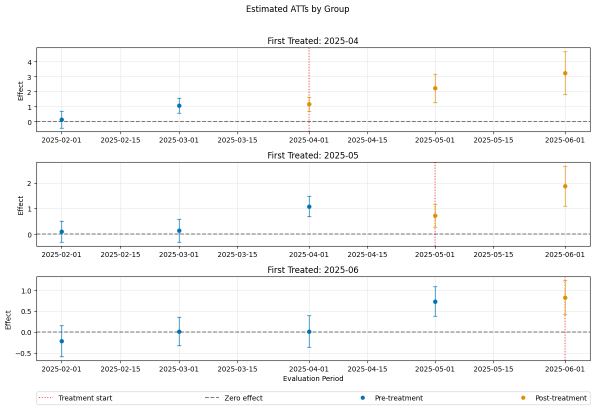
The effects are obviously biased. To include anticipation periods, one can adjust the anticipation_periods parameter. Correspondingly, the outcome regression (and not yet treated units) are adjusted.
[33]:
dml_obj_anticipation = DoubleMLDIDMulti(dml_data_anticipation, **(default_args| {"anticipation_periods": 1}))
dml_obj_anticipation.fit()
dml_obj_anticipation.bootstrap(n_rep_boot=5000)
dml_obj_anticipation.plot_effects()
/opt/hostedtoolcache/Python/3.12.13/x64/lib/python3.12/site-packages/sklearn/utils/validation.py:2739: UserWarning: X does not have valid feature names, but LGBMRegressor was fitted with feature names
  warnings.warn(
/opt/hostedtoolcache/Python/3.12.13/x64/lib/python3.12/site-packages/sklearn/utils/validation.py:2739: UserWarning: X does not have valid feature names, but LGBMRegressor was fitted with feature names
  warnings.warn(
/opt/hostedtoolcache/Python/3.12.13/x64/lib/python3.12/site-packages/sklearn/utils/validation.py:2739: UserWarning: X does not have valid feature names, but LGBMRegressor was fitted with feature names
  warnings.warn(
/opt/hostedtoolcache/Python/3.12.13/x64/lib/python3.12/site-packages/sklearn/utils/validation.py:2739: UserWarning: X does not have valid feature names, but LGBMRegressor was fitted with feature names
  warnings.warn(
/opt/hostedtoolcache/Python/3.12.13/x64/lib/python3.12/site-packages/sklearn/utils/validation.py:2739: UserWarning: X does not have valid feature names, but LGBMRegressor was fitted with feature names
  warnings.warn(
/opt/hostedtoolcache/Python/3.12.13/x64/lib/python3.12/site-packages/sklearn/utils/validation.py:2739: UserWarning: X does not have valid feature names, but LGBMRegressor was fitted with feature names
  warnings.warn(
/opt/hostedtoolcache/Python/3.12.13/x64/lib/python3.12/site-packages/sklearn/utils/validation.py:2739: UserWarning: X does not have valid feature names, but LGBMRegressor was fitted with feature names
  warnings.warn(
/opt/hostedtoolcache/Python/3.12.13/x64/lib/python3.12/site-packages/sklearn/utils/validation.py:2739: UserWarning: X does not have valid feature names, but LGBMRegressor was fitted with feature names
  warnings.warn(
/opt/hostedtoolcache/Python/3.12.13/x64/lib/python3.12/site-packages/sklearn/utils/validation.py:2739: UserWarning: X does not have valid feature names, but LGBMRegressor was fitted with feature names
  warnings.warn(
/opt/hostedtoolcache/Python/3.12.13/x64/lib/python3.12/site-packages/sklearn/utils/validation.py:2739: UserWarning: X does not have valid feature names, but LGBMRegressor was fitted with feature names
  warnings.warn(
/opt/hostedtoolcache/Python/3.12.13/x64/lib/python3.12/site-packages/sklearn/utils/validation.py:2739: UserWarning: X does not have valid feature names, but LGBMClassifier was fitted with feature names
  warnings.warn(
/opt/hostedtoolcache/Python/3.12.13/x64/lib/python3.12/site-packages/sklearn/utils/validation.py:2739: UserWarning: X does not have valid feature names, but LGBMClassifier was fitted with feature names
  warnings.warn(
/opt/hostedtoolcache/Python/3.12.13/x64/lib/python3.12/site-packages/sklearn/utils/validation.py:2739: UserWarning: X does not have valid feature names, but LGBMClassifier was fitted with feature names
  warnings.warn(
/opt/hostedtoolcache/Python/3.12.13/x64/lib/python3.12/site-packages/sklearn/utils/validation.py:2739: UserWarning: X does not have valid feature names, but LGBMClassifier was fitted with feature names
  warnings.warn(
/opt/hostedtoolcache/Python/3.12.13/x64/lib/python3.12/site-packages/sklearn/utils/validation.py:2739: UserWarning: X does not have valid feature names, but LGBMClassifier was fitted with feature names
  warnings.warn(
/opt/hostedtoolcache/Python/3.12.13/x64/lib/python3.12/site-packages/sklearn/utils/validation.py:2739: UserWarning: X does not have valid feature names, but LGBMRegressor was fitted with feature names
  warnings.warn(
/opt/hostedtoolcache/Python/3.12.13/x64/lib/python3.12/site-packages/sklearn/utils/validation.py:2739: UserWarning: X does not have valid feature names, but LGBMRegressor was fitted with feature names
  warnings.warn(
/opt/hostedtoolcache/Python/3.12.13/x64/lib/python3.12/site-packages/sklearn/utils/validation.py:2739: UserWarning: X does not have valid feature names, but LGBMRegressor was fitted with feature names
  warnings.warn(
/opt/hostedtoolcache/Python/3.12.13/x64/lib/python3.12/site-packages/sklearn/utils/validation.py:2739: UserWarning: X does not have valid feature names, but LGBMRegressor was fitted with feature names
  warnings.warn(
/opt/hostedtoolcache/Python/3.12.13/x64/lib/python3.12/site-packages/sklearn/utils/validation.py:2739: UserWarning: X does not have valid feature names, but LGBMRegressor was fitted with feature names
  warnings.warn(
/opt/hostedtoolcache/Python/3.12.13/x64/lib/python3.12/site-packages/sklearn/utils/validation.py:2739: UserWarning: X does not have valid feature names, but LGBMRegressor was fitted with feature names
  warnings.warn(
/opt/hostedtoolcache/Python/3.12.13/x64/lib/python3.12/site-packages/sklearn/utils/validation.py:2739: UserWarning: X does not have valid feature names, but LGBMRegressor was fitted with feature names
  warnings.warn(
/opt/hostedtoolcache/Python/3.12.13/x64/lib/python3.12/site-packages/sklearn/utils/validation.py:2739: UserWarning: X does not have valid feature names, but LGBMRegressor was fitted with feature names
  warnings.warn(
/opt/hostedtoolcache/Python/3.12.13/x64/lib/python3.12/site-packages/sklearn/utils/validation.py:2739: UserWarning: X does not have valid feature names, but LGBMRegressor was fitted with feature names
  warnings.warn(
/opt/hostedtoolcache/Python/3.12.13/x64/lib/python3.12/site-packages/sklearn/utils/validation.py:2739: UserWarning: X does not have valid feature names, but LGBMRegressor was fitted with feature names
  warnings.warn(
/opt/hostedtoolcache/Python/3.12.13/x64/lib/python3.12/site-packages/sklearn/utils/validation.py:2739: UserWarning: X does not have valid feature names, but LGBMClassifier was fitted with feature names
  warnings.warn(
/opt/hostedtoolcache/Python/3.12.13/x64/lib/python3.12/site-packages/sklearn/utils/validation.py:2739: UserWarning: X does not have valid feature names, but LGBMClassifier was fitted with feature names
  warnings.warn(
/opt/hostedtoolcache/Python/3.12.13/x64/lib/python3.12/site-packages/sklearn/utils/validation.py:2739: UserWarning: X does not have valid feature names, but LGBMClassifier was fitted with feature names
  warnings.warn(
/opt/hostedtoolcache/Python/3.12.13/x64/lib/python3.12/site-packages/sklearn/utils/validation.py:2739: UserWarning: X does not have valid feature names, but LGBMClassifier was fitted with feature names
  warnings.warn(
/opt/hostedtoolcache/Python/3.12.13/x64/lib/python3.12/site-packages/sklearn/utils/validation.py:2739: UserWarning: X does not have valid feature names, but LGBMClassifier was fitted with feature names
  warnings.warn(
/opt/hostedtoolcache/Python/3.12.13/x64/lib/python3.12/site-packages/sklearn/utils/validation.py:2739: UserWarning: X does not have valid feature names, but LGBMRegressor was fitted with feature names
  warnings.warn(
/opt/hostedtoolcache/Python/3.12.13/x64/lib/python3.12/site-packages/sklearn/utils/validation.py:2739: UserWarning: X does not have valid feature names, but LGBMRegressor was fitted with feature names
  warnings.warn(
/opt/hostedtoolcache/Python/3.12.13/x64/lib/python3.12/site-packages/sklearn/utils/validation.py:2739: UserWarning: X does not have valid feature names, but LGBMRegressor was fitted with feature names
  warnings.warn(
/opt/hostedtoolcache/Python/3.12.13/x64/lib/python3.12/site-packages/sklearn/utils/validation.py:2739: UserWarning: X does not have valid feature names, but LGBMRegressor was fitted with feature names
  warnings.warn(
/opt/hostedtoolcache/Python/3.12.13/x64/lib/python3.12/site-packages/sklearn/utils/validation.py:2739: UserWarning: X does not have valid feature names, but LGBMRegressor was fitted with feature names
  warnings.warn(
/opt/hostedtoolcache/Python/3.12.13/x64/lib/python3.12/site-packages/sklearn/utils/validation.py:2739: UserWarning: X does not have valid feature names, but LGBMRegressor was fitted with feature names
  warnings.warn(
/opt/hostedtoolcache/Python/3.12.13/x64/lib/python3.12/site-packages/sklearn/utils/validation.py:2739: UserWarning: X does not have valid feature names, but LGBMRegressor was fitted with feature names
  warnings.warn(
/opt/hostedtoolcache/Python/3.12.13/x64/lib/python3.12/site-packages/sklearn/utils/validation.py:2739: UserWarning: X does not have valid feature names, but LGBMRegressor was fitted with feature names
  warnings.warn(
/opt/hostedtoolcache/Python/3.12.13/x64/lib/python3.12/site-packages/sklearn/utils/validation.py:2739: UserWarning: X does not have valid feature names, but LGBMRegressor was fitted with feature names
  warnings.warn(
/opt/hostedtoolcache/Python/3.12.13/x64/lib/python3.12/site-packages/sklearn/utils/validation.py:2739: UserWarning: X does not have valid feature names, but LGBMRegressor was fitted with feature names
  warnings.warn(
/opt/hostedtoolcache/Python/3.12.13/x64/lib/python3.12/site-packages/sklearn/utils/validation.py:2739: UserWarning: X does not have valid feature names, but LGBMClassifier was fitted with feature names
  warnings.warn(
/opt/hostedtoolcache/Python/3.12.13/x64/lib/python3.12/site-packages/sklearn/utils/validation.py:2739: UserWarning: X does not have valid feature names, but LGBMClassifier was fitted with feature names
  warnings.warn(
/opt/hostedtoolcache/Python/3.12.13/x64/lib/python3.12/site-packages/sklearn/utils/validation.py:2739: UserWarning: X does not have valid feature names, but LGBMClassifier was fitted with feature names
  warnings.warn(
/opt/hostedtoolcache/Python/3.12.13/x64/lib/python3.12/site-packages/sklearn/utils/validation.py:2739: UserWarning: X does not have valid feature names, but LGBMClassifier was fitted with feature names
  warnings.warn(
/opt/hostedtoolcache/Python/3.12.13/x64/lib/python3.12/site-packages/sklearn/utils/validation.py:2739: UserWarning: X does not have valid feature names, but LGBMClassifier was fitted with feature names
  warnings.warn(
/opt/hostedtoolcache/Python/3.12.13/x64/lib/python3.12/site-packages/sklearn/utils/validation.py:2739: UserWarning: X does not have valid feature names, but LGBMRegressor was fitted with feature names
  warnings.warn(
/opt/hostedtoolcache/Python/3.12.13/x64/lib/python3.12/site-packages/sklearn/utils/validation.py:2739: UserWarning: X does not have valid feature names, but LGBMRegressor was fitted with feature names
  warnings.warn(
/opt/hostedtoolcache/Python/3.12.13/x64/lib/python3.12/site-packages/sklearn/utils/validation.py:2739: UserWarning: X does not have valid feature names, but LGBMRegressor was fitted with feature names
  warnings.warn(
/opt/hostedtoolcache/Python/3.12.13/x64/lib/python3.12/site-packages/sklearn/utils/validation.py:2739: UserWarning: X does not have valid feature names, but LGBMRegressor was fitted with feature names
  warnings.warn(
/opt/hostedtoolcache/Python/3.12.13/x64/lib/python3.12/site-packages/sklearn/utils/validation.py:2739: UserWarning: X does not have valid feature names, but LGBMRegressor was fitted with feature names
  warnings.warn(
/opt/hostedtoolcache/Python/3.12.13/x64/lib/python3.12/site-packages/sklearn/utils/validation.py:2739: UserWarning: X does not have valid feature names, but LGBMRegressor was fitted with feature names
  warnings.warn(
/opt/hostedtoolcache/Python/3.12.13/x64/lib/python3.12/site-packages/sklearn/utils/validation.py:2739: UserWarning: X does not have valid feature names, but LGBMRegressor was fitted with feature names
  warnings.warn(
/opt/hostedtoolcache/Python/3.12.13/x64/lib/python3.12/site-packages/sklearn/utils/validation.py:2739: UserWarning: X does not have valid feature names, but LGBMRegressor was fitted with feature names
  warnings.warn(
/opt/hostedtoolcache/Python/3.12.13/x64/lib/python3.12/site-packages/sklearn/utils/validation.py:2739: UserWarning: X does not have valid feature names, but LGBMRegressor was fitted with feature names
  warnings.warn(
/opt/hostedtoolcache/Python/3.12.13/x64/lib/python3.12/site-packages/sklearn/utils/validation.py:2739: UserWarning: X does not have valid feature names, but LGBMRegressor was fitted with feature names
  warnings.warn(
/opt/hostedtoolcache/Python/3.12.13/x64/lib/python3.12/site-packages/sklearn/utils/validation.py:2739: UserWarning: X does not have valid feature names, but LGBMClassifier was fitted with feature names
  warnings.warn(
/opt/hostedtoolcache/Python/3.12.13/x64/lib/python3.12/site-packages/sklearn/utils/validation.py:2739: UserWarning: X does not have valid feature names, but LGBMClassifier was fitted with feature names
  warnings.warn(
/opt/hostedtoolcache/Python/3.12.13/x64/lib/python3.12/site-packages/sklearn/utils/validation.py:2739: UserWarning: X does not have valid feature names, but LGBMClassifier was fitted with feature names
  warnings.warn(
/opt/hostedtoolcache/Python/3.12.13/x64/lib/python3.12/site-packages/sklearn/utils/validation.py:2739: UserWarning: X does not have valid feature names, but LGBMClassifier was fitted with feature names
  warnings.warn(
/opt/hostedtoolcache/Python/3.12.13/x64/lib/python3.12/site-packages/sklearn/utils/validation.py:2739: UserWarning: X does not have valid feature names, but LGBMClassifier was fitted with feature names
  warnings.warn(
/opt/hostedtoolcache/Python/3.12.13/x64/lib/python3.12/site-packages/sklearn/utils/validation.py:2739: UserWarning: X does not have valid feature names, but LGBMRegressor was fitted with feature names
  warnings.warn(
/opt/hostedtoolcache/Python/3.12.13/x64/lib/python3.12/site-packages/sklearn/utils/validation.py:2739: UserWarning: X does not have valid feature names, but LGBMRegressor was fitted with feature names
  warnings.warn(
/opt/hostedtoolcache/Python/3.12.13/x64/lib/python3.12/site-packages/sklearn/utils/validation.py:2739: UserWarning: X does not have valid feature names, but LGBMRegressor was fitted with feature names
  warnings.warn(
/opt/hostedtoolcache/Python/3.12.13/x64/lib/python3.12/site-packages/sklearn/utils/validation.py:2739: UserWarning: X does not have valid feature names, but LGBMRegressor was fitted with feature names
  warnings.warn(
/opt/hostedtoolcache/Python/3.12.13/x64/lib/python3.12/site-packages/sklearn/utils/validation.py:2739: UserWarning: X does not have valid feature names, but LGBMRegressor was fitted with feature names
  warnings.warn(
/opt/hostedtoolcache/Python/3.12.13/x64/lib/python3.12/site-packages/sklearn/utils/validation.py:2739: UserWarning: X does not have valid feature names, but LGBMRegressor was fitted with feature names
  warnings.warn(
/opt/hostedtoolcache/Python/3.12.13/x64/lib/python3.12/site-packages/sklearn/utils/validation.py:2739: UserWarning: X does not have valid feature names, but LGBMRegressor was fitted with feature names
  warnings.warn(
/opt/hostedtoolcache/Python/3.12.13/x64/lib/python3.12/site-packages/sklearn/utils/validation.py:2739: UserWarning: X does not have valid feature names, but LGBMRegressor was fitted with feature names
  warnings.warn(
/opt/hostedtoolcache/Python/3.12.13/x64/lib/python3.12/site-packages/sklearn/utils/validation.py:2739: UserWarning: X does not have valid feature names, but LGBMRegressor was fitted with feature names
  warnings.warn(
/opt/hostedtoolcache/Python/3.12.13/x64/lib/python3.12/site-packages/sklearn/utils/validation.py:2739: UserWarning: X does not have valid feature names, but LGBMRegressor was fitted with feature names
  warnings.warn(
/opt/hostedtoolcache/Python/3.12.13/x64/lib/python3.12/site-packages/sklearn/utils/validation.py:2739: UserWarning: X does not have valid feature names, but LGBMClassifier was fitted with feature names
  warnings.warn(
/opt/hostedtoolcache/Python/3.12.13/x64/lib/python3.12/site-packages/sklearn/utils/validation.py:2739: UserWarning: X does not have valid feature names, but LGBMClassifier was fitted with feature names
  warnings.warn(
/opt/hostedtoolcache/Python/3.12.13/x64/lib/python3.12/site-packages/sklearn/utils/validation.py:2739: UserWarning: X does not have valid feature names, but LGBMClassifier was fitted with feature names
  warnings.warn(
/opt/hostedtoolcache/Python/3.12.13/x64/lib/python3.12/site-packages/sklearn/utils/validation.py:2739: UserWarning: X does not have valid feature names, but LGBMClassifier was fitted with feature names
  warnings.warn(
/opt/hostedtoolcache/Python/3.12.13/x64/lib/python3.12/site-packages/sklearn/utils/validation.py:2739: UserWarning: X does not have valid feature names, but LGBMClassifier was fitted with feature names
  warnings.warn(
/opt/hostedtoolcache/Python/3.12.13/x64/lib/python3.12/site-packages/sklearn/utils/validation.py:2739: UserWarning: X does not have valid feature names, but LGBMRegressor was fitted with feature names
  warnings.warn(
/opt/hostedtoolcache/Python/3.12.13/x64/lib/python3.12/site-packages/sklearn/utils/validation.py:2739: UserWarning: X does not have valid feature names, but LGBMRegressor was fitted with feature names
  warnings.warn(
/opt/hostedtoolcache/Python/3.12.13/x64/lib/python3.12/site-packages/sklearn/utils/validation.py:2739: UserWarning: X does not have valid feature names, but LGBMRegressor was fitted with feature names
  warnings.warn(
/opt/hostedtoolcache/Python/3.12.13/x64/lib/python3.12/site-packages/sklearn/utils/validation.py:2739: UserWarning: X does not have valid feature names, but LGBMRegressor was fitted with feature names
  warnings.warn(
/opt/hostedtoolcache/Python/3.12.13/x64/lib/python3.12/site-packages/sklearn/utils/validation.py:2739: UserWarning: X does not have valid feature names, but LGBMRegressor was fitted with feature names
  warnings.warn(
/opt/hostedtoolcache/Python/3.12.13/x64/lib/python3.12/site-packages/sklearn/utils/validation.py:2739: UserWarning: X does not have valid feature names, but LGBMRegressor was fitted with feature names
  warnings.warn(
/opt/hostedtoolcache/Python/3.12.13/x64/lib/python3.12/site-packages/sklearn/utils/validation.py:2739: UserWarning: X does not have valid feature names, but LGBMRegressor was fitted with feature names
  warnings.warn(
/opt/hostedtoolcache/Python/3.12.13/x64/lib/python3.12/site-packages/sklearn/utils/validation.py:2739: UserWarning: X does not have valid feature names, but LGBMRegressor was fitted with feature names
  warnings.warn(
/opt/hostedtoolcache/Python/3.12.13/x64/lib/python3.12/site-packages/sklearn/utils/validation.py:2739: UserWarning: X does not have valid feature names, but LGBMRegressor was fitted with feature names
  warnings.warn(
/opt/hostedtoolcache/Python/3.12.13/x64/lib/python3.12/site-packages/sklearn/utils/validation.py:2739: UserWarning: X does not have valid feature names, but LGBMRegressor was fitted with feature names
  warnings.warn(
/opt/hostedtoolcache/Python/3.12.13/x64/lib/python3.12/site-packages/sklearn/utils/validation.py:2739: UserWarning: X does not have valid feature names, but LGBMClassifier was fitted with feature names
  warnings.warn(
/opt/hostedtoolcache/Python/3.12.13/x64/lib/python3.12/site-packages/sklearn/utils/validation.py:2739: UserWarning: X does not have valid feature names, but LGBMClassifier was fitted with feature names
  warnings.warn(
/opt/hostedtoolcache/Python/3.12.13/x64/lib/python3.12/site-packages/sklearn/utils/validation.py:2739: UserWarning: X does not have valid feature names, but LGBMClassifier was fitted with feature names
  warnings.warn(
/opt/hostedtoolcache/Python/3.12.13/x64/lib/python3.12/site-packages/sklearn/utils/validation.py:2739: UserWarning: X does not have valid feature names, but LGBMClassifier was fitted with feature names
  warnings.warn(
/opt/hostedtoolcache/Python/3.12.13/x64/lib/python3.12/site-packages/sklearn/utils/validation.py:2739: UserWarning: X does not have valid feature names, but LGBMClassifier was fitted with feature names
  warnings.warn(
/opt/hostedtoolcache/Python/3.12.13/x64/lib/python3.12/site-packages/sklearn/utils/validation.py:2739: UserWarning: X does not have valid feature names, but LGBMRegressor was fitted with feature names
  warnings.warn(
/opt/hostedtoolcache/Python/3.12.13/x64/lib/python3.12/site-packages/sklearn/utils/validation.py:2739: UserWarning: X does not have valid feature names, but LGBMRegressor was fitted with feature names
  warnings.warn(
/opt/hostedtoolcache/Python/3.12.13/x64/lib/python3.12/site-packages/sklearn/utils/validation.py:2739: UserWarning: X does not have valid feature names, but LGBMRegressor was fitted with feature names
  warnings.warn(
/opt/hostedtoolcache/Python/3.12.13/x64/lib/python3.12/site-packages/sklearn/utils/validation.py:2739: UserWarning: X does not have valid feature names, but LGBMRegressor was fitted with feature names
  warnings.warn(
/opt/hostedtoolcache/Python/3.12.13/x64/lib/python3.12/site-packages/sklearn/utils/validation.py:2739: UserWarning: X does not have valid feature names, but LGBMRegressor was fitted with feature names
  warnings.warn(
/opt/hostedtoolcache/Python/3.12.13/x64/lib/python3.12/site-packages/sklearn/utils/validation.py:2739: UserWarning: X does not have valid feature names, but LGBMRegressor was fitted with feature names
  warnings.warn(
/opt/hostedtoolcache/Python/3.12.13/x64/lib/python3.12/site-packages/sklearn/utils/validation.py:2739: UserWarning: X does not have valid feature names, but LGBMRegressor was fitted with feature names
  warnings.warn(
/opt/hostedtoolcache/Python/3.12.13/x64/lib/python3.12/site-packages/sklearn/utils/validation.py:2739: UserWarning: X does not have valid feature names, but LGBMRegressor was fitted with feature names
  warnings.warn(
/opt/hostedtoolcache/Python/3.12.13/x64/lib/python3.12/site-packages/sklearn/utils/validation.py:2739: UserWarning: X does not have valid feature names, but LGBMRegressor was fitted with feature names
  warnings.warn(
/opt/hostedtoolcache/Python/3.12.13/x64/lib/python3.12/site-packages/sklearn/utils/validation.py:2739: UserWarning: X does not have valid feature names, but LGBMRegressor was fitted with feature names
  warnings.warn(
/opt/hostedtoolcache/Python/3.12.13/x64/lib/python3.12/site-packages/sklearn/utils/validation.py:2739: UserWarning: X does not have valid feature names, but LGBMClassifier was fitted with feature names
  warnings.warn(
/opt/hostedtoolcache/Python/3.12.13/x64/lib/python3.12/site-packages/sklearn/utils/validation.py:2739: UserWarning: X does not have valid feature names, but LGBMClassifier was fitted with feature names
  warnings.warn(
/opt/hostedtoolcache/Python/3.12.13/x64/lib/python3.12/site-packages/sklearn/utils/validation.py:2739: UserWarning: X does not have valid feature names, but LGBMClassifier was fitted with feature names
  warnings.warn(
/opt/hostedtoolcache/Python/3.12.13/x64/lib/python3.12/site-packages/sklearn/utils/validation.py:2739: UserWarning: X does not have valid feature names, but LGBMClassifier was fitted with feature names
  warnings.warn(
/opt/hostedtoolcache/Python/3.12.13/x64/lib/python3.12/site-packages/sklearn/utils/validation.py:2739: UserWarning: X does not have valid feature names, but LGBMClassifier was fitted with feature names
  warnings.warn(
/opt/hostedtoolcache/Python/3.12.13/x64/lib/python3.12/site-packages/sklearn/utils/validation.py:2739: UserWarning: X does not have valid feature names, but LGBMRegressor was fitted with feature names
  warnings.warn(
/opt/hostedtoolcache/Python/3.12.13/x64/lib/python3.12/site-packages/sklearn/utils/validation.py:2739: UserWarning: X does not have valid feature names, but LGBMRegressor was fitted with feature names
  warnings.warn(
/opt/hostedtoolcache/Python/3.12.13/x64/lib/python3.12/site-packages/sklearn/utils/validation.py:2739: UserWarning: X does not have valid feature names, but LGBMRegressor was fitted with feature names
  warnings.warn(
/opt/hostedtoolcache/Python/3.12.13/x64/lib/python3.12/site-packages/sklearn/utils/validation.py:2739: UserWarning: X does not have valid feature names, but LGBMRegressor was fitted with feature names
  warnings.warn(
/opt/hostedtoolcache/Python/3.12.13/x64/lib/python3.12/site-packages/sklearn/utils/validation.py:2739: UserWarning: X does not have valid feature names, but LGBMRegressor was fitted with feature names
  warnings.warn(
/opt/hostedtoolcache/Python/3.12.13/x64/lib/python3.12/site-packages/sklearn/utils/validation.py:2739: UserWarning: X does not have valid feature names, but LGBMRegressor was fitted with feature names
  warnings.warn(
/opt/hostedtoolcache/Python/3.12.13/x64/lib/python3.12/site-packages/sklearn/utils/validation.py:2739: UserWarning: X does not have valid feature names, but LGBMRegressor was fitted with feature names
  warnings.warn(
/opt/hostedtoolcache/Python/3.12.13/x64/lib/python3.12/site-packages/sklearn/utils/validation.py:2739: UserWarning: X does not have valid feature names, but LGBMRegressor was fitted with feature names
  warnings.warn(
/opt/hostedtoolcache/Python/3.12.13/x64/lib/python3.12/site-packages/sklearn/utils/validation.py:2739: UserWarning: X does not have valid feature names, but LGBMRegressor was fitted with feature names
  warnings.warn(
/opt/hostedtoolcache/Python/3.12.13/x64/lib/python3.12/site-packages/sklearn/utils/validation.py:2739: UserWarning: X does not have valid feature names, but LGBMRegressor was fitted with feature names
  warnings.warn(
/opt/hostedtoolcache/Python/3.12.13/x64/lib/python3.12/site-packages/sklearn/utils/validation.py:2739: UserWarning: X does not have valid feature names, but LGBMClassifier was fitted with feature names
  warnings.warn(
/opt/hostedtoolcache/Python/3.12.13/x64/lib/python3.12/site-packages/sklearn/utils/validation.py:2739: UserWarning: X does not have valid feature names, but LGBMClassifier was fitted with feature names
  warnings.warn(
/opt/hostedtoolcache/Python/3.12.13/x64/lib/python3.12/site-packages/sklearn/utils/validation.py:2739: UserWarning: X does not have valid feature names, but LGBMClassifier was fitted with feature names
  warnings.warn(
/opt/hostedtoolcache/Python/3.12.13/x64/lib/python3.12/site-packages/sklearn/utils/validation.py:2739: UserWarning: X does not have valid feature names, but LGBMClassifier was fitted with feature names
  warnings.warn(
/opt/hostedtoolcache/Python/3.12.13/x64/lib/python3.12/site-packages/sklearn/utils/validation.py:2739: UserWarning: X does not have valid feature names, but LGBMClassifier was fitted with feature names
  warnings.warn(
/opt/hostedtoolcache/Python/3.12.13/x64/lib/python3.12/site-packages/sklearn/utils/validation.py:2739: UserWarning: X does not have valid feature names, but LGBMRegressor was fitted with feature names
  warnings.warn(
/opt/hostedtoolcache/Python/3.12.13/x64/lib/python3.12/site-packages/sklearn/utils/validation.py:2739: UserWarning: X does not have valid feature names, but LGBMRegressor was fitted with feature names
  warnings.warn(
/opt/hostedtoolcache/Python/3.12.13/x64/lib/python3.12/site-packages/sklearn/utils/validation.py:2739: UserWarning: X does not have valid feature names, but LGBMRegressor was fitted with feature names
  warnings.warn(
/opt/hostedtoolcache/Python/3.12.13/x64/lib/python3.12/site-packages/sklearn/utils/validation.py:2739: UserWarning: X does not have valid feature names, but LGBMRegressor was fitted with feature names
  warnings.warn(
/opt/hostedtoolcache/Python/3.12.13/x64/lib/python3.12/site-packages/sklearn/utils/validation.py:2739: UserWarning: X does not have valid feature names, but LGBMRegressor was fitted with feature names
  warnings.warn(
/opt/hostedtoolcache/Python/3.12.13/x64/lib/python3.12/site-packages/sklearn/utils/validation.py:2739: UserWarning: X does not have valid feature names, but LGBMRegressor was fitted with feature names
  warnings.warn(
/opt/hostedtoolcache/Python/3.12.13/x64/lib/python3.12/site-packages/sklearn/utils/validation.py:2739: UserWarning: X does not have valid feature names, but LGBMRegressor was fitted with feature names
  warnings.warn(
/opt/hostedtoolcache/Python/3.12.13/x64/lib/python3.12/site-packages/sklearn/utils/validation.py:2739: UserWarning: X does not have valid feature names, but LGBMRegressor was fitted with feature names
  warnings.warn(
/opt/hostedtoolcache/Python/3.12.13/x64/lib/python3.12/site-packages/sklearn/utils/validation.py:2739: UserWarning: X does not have valid feature names, but LGBMRegressor was fitted with feature names
  warnings.warn(
/opt/hostedtoolcache/Python/3.12.13/x64/lib/python3.12/site-packages/sklearn/utils/validation.py:2739: UserWarning: X does not have valid feature names, but LGBMRegressor was fitted with feature names
  warnings.warn(
/opt/hostedtoolcache/Python/3.12.13/x64/lib/python3.12/site-packages/sklearn/utils/validation.py:2739: UserWarning: X does not have valid feature names, but LGBMClassifier was fitted with feature names
  warnings.warn(
/opt/hostedtoolcache/Python/3.12.13/x64/lib/python3.12/site-packages/sklearn/utils/validation.py:2739: UserWarning: X does not have valid feature names, but LGBMClassifier was fitted with feature names
  warnings.warn(
/opt/hostedtoolcache/Python/3.12.13/x64/lib/python3.12/site-packages/sklearn/utils/validation.py:2739: UserWarning: X does not have valid feature names, but LGBMClassifier was fitted with feature names
  warnings.warn(
/opt/hostedtoolcache/Python/3.12.13/x64/lib/python3.12/site-packages/sklearn/utils/validation.py:2739: UserWarning: X does not have valid feature names, but LGBMClassifier was fitted with feature names
  warnings.warn(
/opt/hostedtoolcache/Python/3.12.13/x64/lib/python3.12/site-packages/sklearn/utils/validation.py:2739: UserWarning: X does not have valid feature names, but LGBMClassifier was fitted with feature names
  warnings.warn(
/opt/hostedtoolcache/Python/3.12.13/x64/lib/python3.12/site-packages/sklearn/utils/validation.py:2739: UserWarning: X does not have valid feature names, but LGBMRegressor was fitted with feature names
  warnings.warn(
/opt/hostedtoolcache/Python/3.12.13/x64/lib/python3.12/site-packages/sklearn/utils/validation.py:2739: UserWarning: X does not have valid feature names, but LGBMRegressor was fitted with feature names
  warnings.warn(
/opt/hostedtoolcache/Python/3.12.13/x64/lib/python3.12/site-packages/sklearn/utils/validation.py:2739: UserWarning: X does not have valid feature names, but LGBMRegressor was fitted with feature names
  warnings.warn(
/opt/hostedtoolcache/Python/3.12.13/x64/lib/python3.12/site-packages/sklearn/utils/validation.py:2739: UserWarning: X does not have valid feature names, but LGBMRegressor was fitted with feature names
  warnings.warn(
/opt/hostedtoolcache/Python/3.12.13/x64/lib/python3.12/site-packages/sklearn/utils/validation.py:2739: UserWarning: X does not have valid feature names, but LGBMRegressor was fitted with feature names
  warnings.warn(
/opt/hostedtoolcache/Python/3.12.13/x64/lib/python3.12/site-packages/sklearn/utils/validation.py:2739: UserWarning: X does not have valid feature names, but LGBMRegressor was fitted with feature names
  warnings.warn(
/opt/hostedtoolcache/Python/3.12.13/x64/lib/python3.12/site-packages/sklearn/utils/validation.py:2739: UserWarning: X does not have valid feature names, but LGBMRegressor was fitted with feature names
  warnings.warn(
/opt/hostedtoolcache/Python/3.12.13/x64/lib/python3.12/site-packages/sklearn/utils/validation.py:2739: UserWarning: X does not have valid feature names, but LGBMRegressor was fitted with feature names
  warnings.warn(
/opt/hostedtoolcache/Python/3.12.13/x64/lib/python3.12/site-packages/sklearn/utils/validation.py:2739: UserWarning: X does not have valid feature names, but LGBMRegressor was fitted with feature names
  warnings.warn(
/opt/hostedtoolcache/Python/3.12.13/x64/lib/python3.12/site-packages/sklearn/utils/validation.py:2739: UserWarning: X does not have valid feature names, but LGBMRegressor was fitted with feature names
  warnings.warn(
/opt/hostedtoolcache/Python/3.12.13/x64/lib/python3.12/site-packages/sklearn/utils/validation.py:2739: UserWarning: X does not have valid feature names, but LGBMClassifier was fitted with feature names
  warnings.warn(
/opt/hostedtoolcache/Python/3.12.13/x64/lib/python3.12/site-packages/sklearn/utils/validation.py:2739: UserWarning: X does not have valid feature names, but LGBMClassifier was fitted with feature names
  warnings.warn(
/opt/hostedtoolcache/Python/3.12.13/x64/lib/python3.12/site-packages/sklearn/utils/validation.py:2739: UserWarning: X does not have valid feature names, but LGBMClassifier was fitted with feature names
  warnings.warn(
/opt/hostedtoolcache/Python/3.12.13/x64/lib/python3.12/site-packages/sklearn/utils/validation.py:2739: UserWarning: X does not have valid feature names, but LGBMClassifier was fitted with feature names
  warnings.warn(
/opt/hostedtoolcache/Python/3.12.13/x64/lib/python3.12/site-packages/sklearn/utils/validation.py:2739: UserWarning: X does not have valid feature names, but LGBMClassifier was fitted with feature names
  warnings.warn(
/opt/hostedtoolcache/Python/3.12.13/x64/lib/python3.12/site-packages/sklearn/utils/validation.py:2739: UserWarning: X does not have valid feature names, but LGBMRegressor was fitted with feature names
  warnings.warn(
/opt/hostedtoolcache/Python/3.12.13/x64/lib/python3.12/site-packages/sklearn/utils/validation.py:2739: UserWarning: X does not have valid feature names, but LGBMRegressor was fitted with feature names
  warnings.warn(
/opt/hostedtoolcache/Python/3.12.13/x64/lib/python3.12/site-packages/sklearn/utils/validation.py:2739: UserWarning: X does not have valid feature names, but LGBMRegressor was fitted with feature names
  warnings.warn(
/opt/hostedtoolcache/Python/3.12.13/x64/lib/python3.12/site-packages/sklearn/utils/validation.py:2739: UserWarning: X does not have valid feature names, but LGBMRegressor was fitted with feature names
  warnings.warn(
/opt/hostedtoolcache/Python/3.12.13/x64/lib/python3.12/site-packages/sklearn/utils/validation.py:2739: UserWarning: X does not have valid feature names, but LGBMRegressor was fitted with feature names
  warnings.warn(
/opt/hostedtoolcache/Python/3.12.13/x64/lib/python3.12/site-packages/sklearn/utils/validation.py:2739: UserWarning: X does not have valid feature names, but LGBMRegressor was fitted with feature names
  warnings.warn(
/opt/hostedtoolcache/Python/3.12.13/x64/lib/python3.12/site-packages/sklearn/utils/validation.py:2739: UserWarning: X does not have valid feature names, but LGBMRegressor was fitted with feature names
  warnings.warn(
/opt/hostedtoolcache/Python/3.12.13/x64/lib/python3.12/site-packages/sklearn/utils/validation.py:2739: UserWarning: X does not have valid feature names, but LGBMRegressor was fitted with feature names
  warnings.warn(
/opt/hostedtoolcache/Python/3.12.13/x64/lib/python3.12/site-packages/sklearn/utils/validation.py:2739: UserWarning: X does not have valid feature names, but LGBMRegressor was fitted with feature names
  warnings.warn(
/opt/hostedtoolcache/Python/3.12.13/x64/lib/python3.12/site-packages/sklearn/utils/validation.py:2739: UserWarning: X does not have valid feature names, but LGBMRegressor was fitted with feature names
  warnings.warn(
/opt/hostedtoolcache/Python/3.12.13/x64/lib/python3.12/site-packages/sklearn/utils/validation.py:2739: UserWarning: X does not have valid feature names, but LGBMClassifier was fitted with feature names
  warnings.warn(
/opt/hostedtoolcache/Python/3.12.13/x64/lib/python3.12/site-packages/sklearn/utils/validation.py:2739: UserWarning: X does not have valid feature names, but LGBMClassifier was fitted with feature names
  warnings.warn(
/opt/hostedtoolcache/Python/3.12.13/x64/lib/python3.12/site-packages/sklearn/utils/validation.py:2739: UserWarning: X does not have valid feature names, but LGBMClassifier was fitted with feature names
  warnings.warn(
/opt/hostedtoolcache/Python/3.12.13/x64/lib/python3.12/site-packages/sklearn/utils/validation.py:2739: UserWarning: X does not have valid feature names, but LGBMClassifier was fitted with feature names
  warnings.warn(
/opt/hostedtoolcache/Python/3.12.13/x64/lib/python3.12/site-packages/sklearn/utils/validation.py:2739: UserWarning: X does not have valid feature names, but LGBMClassifier was fitted with feature names
  warnings.warn(
/opt/hostedtoolcache/Python/3.12.13/x64/lib/python3.12/site-packages/sklearn/utils/validation.py:2739: UserWarning: X does not have valid feature names, but LGBMRegressor was fitted with feature names
  warnings.warn(
/opt/hostedtoolcache/Python/3.12.13/x64/lib/python3.12/site-packages/sklearn/utils/validation.py:2739: UserWarning: X does not have valid feature names, but LGBMRegressor was fitted with feature names
  warnings.warn(
/opt/hostedtoolcache/Python/3.12.13/x64/lib/python3.12/site-packages/sklearn/utils/validation.py:2739: UserWarning: X does not have valid feature names, but LGBMRegressor was fitted with feature names
  warnings.warn(
/opt/hostedtoolcache/Python/3.12.13/x64/lib/python3.12/site-packages/sklearn/utils/validation.py:2739: UserWarning: X does not have valid feature names, but LGBMRegressor was fitted with feature names
  warnings.warn(
/opt/hostedtoolcache/Python/3.12.13/x64/lib/python3.12/site-packages/sklearn/utils/validation.py:2739: UserWarning: X does not have valid feature names, but LGBMRegressor was fitted with feature names
  warnings.warn(
/opt/hostedtoolcache/Python/3.12.13/x64/lib/python3.12/site-packages/sklearn/utils/validation.py:2739: UserWarning: X does not have valid feature names, but LGBMRegressor was fitted with feature names
  warnings.warn(
/opt/hostedtoolcache/Python/3.12.13/x64/lib/python3.12/site-packages/sklearn/utils/validation.py:2739: UserWarning: X does not have valid feature names, but LGBMRegressor was fitted with feature names
  warnings.warn(
/opt/hostedtoolcache/Python/3.12.13/x64/lib/python3.12/site-packages/sklearn/utils/validation.py:2739: UserWarning: X does not have valid feature names, but LGBMRegressor was fitted with feature names
  warnings.warn(
/opt/hostedtoolcache/Python/3.12.13/x64/lib/python3.12/site-packages/sklearn/utils/validation.py:2739: UserWarning: X does not have valid feature names, but LGBMRegressor was fitted with feature names
  warnings.warn(
/opt/hostedtoolcache/Python/3.12.13/x64/lib/python3.12/site-packages/sklearn/utils/validation.py:2739: UserWarning: X does not have valid feature names, but LGBMRegressor was fitted with feature names
  warnings.warn(
/opt/hostedtoolcache/Python/3.12.13/x64/lib/python3.12/site-packages/sklearn/utils/validation.py:2739: UserWarning: X does not have valid feature names, but LGBMClassifier was fitted with feature names
  warnings.warn(
/opt/hostedtoolcache/Python/3.12.13/x64/lib/python3.12/site-packages/sklearn/utils/validation.py:2739: UserWarning: X does not have valid feature names, but LGBMClassifier was fitted with feature names
  warnings.warn(
/opt/hostedtoolcache/Python/3.12.13/x64/lib/python3.12/site-packages/sklearn/utils/validation.py:2739: UserWarning: X does not have valid feature names, but LGBMClassifier was fitted with feature names
  warnings.warn(
/opt/hostedtoolcache/Python/3.12.13/x64/lib/python3.12/site-packages/sklearn/utils/validation.py:2739: UserWarning: X does not have valid feature names, but LGBMClassifier was fitted with feature names
  warnings.warn(
/opt/hostedtoolcache/Python/3.12.13/x64/lib/python3.12/site-packages/sklearn/utils/validation.py:2739: UserWarning: X does not have valid feature names, but LGBMClassifier was fitted with feature names
  warnings.warn(
[33]:
(<Figure size 1200x800 with 4 Axes>,
 [<Axes: title={'center': 'First Treated: 2025-04'}, ylabel='Effect'>,
  <Axes: title={'center': 'First Treated: 2025-05'}, ylabel='Effect'>,
  <Axes: title={'center': 'First Treated: 2025-06'}, xlabel='Evaluation Period', ylabel='Effect'>])
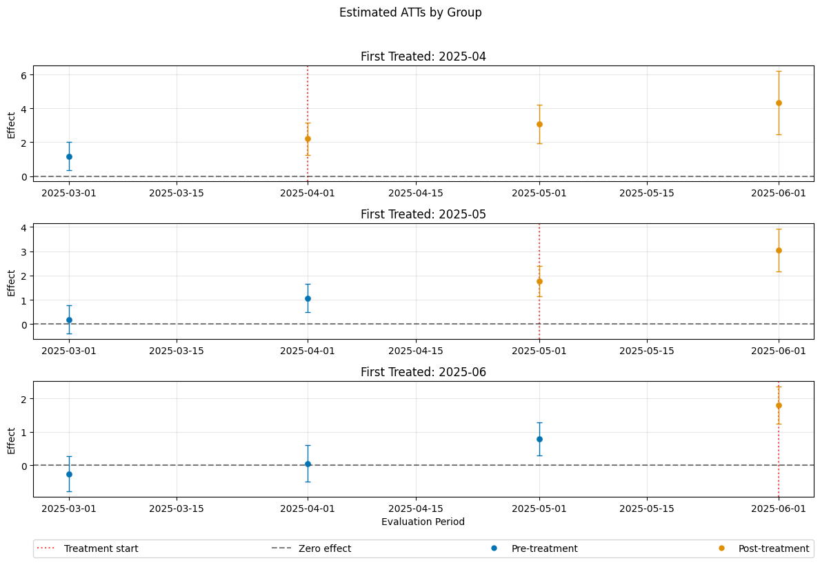
Group-Time Combinations#
The default option gt_combinations="standard" includes all group time values with the specific choice of \(t_\text{pre} = \min(\mathrm{g}, t_\text{eval}) - 1\) (without anticipation) which is the weakest possible parallel trend assumption.
Other options are possible or only specific combinations of \((\mathrm{g},t_\text{pre},t_\text{eval})\).
All Combinations#
The option gt_combinations="all" includes all relevant group time values with \(t_\text{pre} < \min(\mathrm{g}, t_\text{eval})\), including longer parallel trend assumptions. This can result in multiple estimates for the same \(ATT(\mathrm{g},t)\), which have slightly different assumptions (length of parallel trends).
[34]:
dml_obj_all = DoubleMLDIDMulti(dml_data, **(default_args| {"gt_combinations": "all"}))
dml_obj_all.fit()
dml_obj_all.bootstrap(n_rep_boot=5000)
dml_obj_all.plot_effects()
/opt/hostedtoolcache/Python/3.12.13/x64/lib/python3.12/site-packages/sklearn/utils/validation.py:2739: UserWarning: X does not have valid feature names, but LGBMRegressor was fitted with feature names
  warnings.warn(
/opt/hostedtoolcache/Python/3.12.13/x64/lib/python3.12/site-packages/sklearn/utils/validation.py:2739: UserWarning: X does not have valid feature names, but LGBMRegressor was fitted with feature names
  warnings.warn(
/opt/hostedtoolcache/Python/3.12.13/x64/lib/python3.12/site-packages/sklearn/utils/validation.py:2739: UserWarning: X does not have valid feature names, but LGBMRegressor was fitted with feature names
  warnings.warn(
/opt/hostedtoolcache/Python/3.12.13/x64/lib/python3.12/site-packages/sklearn/utils/validation.py:2739: UserWarning: X does not have valid feature names, but LGBMRegressor was fitted with feature names
  warnings.warn(
/opt/hostedtoolcache/Python/3.12.13/x64/lib/python3.12/site-packages/sklearn/utils/validation.py:2739: UserWarning: X does not have valid feature names, but LGBMRegressor was fitted with feature names
  warnings.warn(
/opt/hostedtoolcache/Python/3.12.13/x64/lib/python3.12/site-packages/sklearn/utils/validation.py:2739: UserWarning: X does not have valid feature names, but LGBMRegressor was fitted with feature names
  warnings.warn(
/opt/hostedtoolcache/Python/3.12.13/x64/lib/python3.12/site-packages/sklearn/utils/validation.py:2739: UserWarning: X does not have valid feature names, but LGBMRegressor was fitted with feature names
  warnings.warn(
/opt/hostedtoolcache/Python/3.12.13/x64/lib/python3.12/site-packages/sklearn/utils/validation.py:2739: UserWarning: X does not have valid feature names, but LGBMRegressor was fitted with feature names
  warnings.warn(
/opt/hostedtoolcache/Python/3.12.13/x64/lib/python3.12/site-packages/sklearn/utils/validation.py:2739: UserWarning: X does not have valid feature names, but LGBMRegressor was fitted with feature names
  warnings.warn(
/opt/hostedtoolcache/Python/3.12.13/x64/lib/python3.12/site-packages/sklearn/utils/validation.py:2739: UserWarning: X does not have valid feature names, but LGBMRegressor was fitted with feature names
  warnings.warn(
/opt/hostedtoolcache/Python/3.12.13/x64/lib/python3.12/site-packages/sklearn/utils/validation.py:2739: UserWarning: X does not have valid feature names, but LGBMClassifier was fitted with feature names
  warnings.warn(
/opt/hostedtoolcache/Python/3.12.13/x64/lib/python3.12/site-packages/sklearn/utils/validation.py:2739: UserWarning: X does not have valid feature names, but LGBMClassifier was fitted with feature names
  warnings.warn(
/opt/hostedtoolcache/Python/3.12.13/x64/lib/python3.12/site-packages/sklearn/utils/validation.py:2739: UserWarning: X does not have valid feature names, but LGBMClassifier was fitted with feature names
  warnings.warn(
/opt/hostedtoolcache/Python/3.12.13/x64/lib/python3.12/site-packages/sklearn/utils/validation.py:2739: UserWarning: X does not have valid feature names, but LGBMClassifier was fitted with feature names
  warnings.warn(
/opt/hostedtoolcache/Python/3.12.13/x64/lib/python3.12/site-packages/sklearn/utils/validation.py:2739: UserWarning: X does not have valid feature names, but LGBMClassifier was fitted with feature names
  warnings.warn(
/opt/hostedtoolcache/Python/3.12.13/x64/lib/python3.12/site-packages/sklearn/utils/validation.py:2739: UserWarning: X does not have valid feature names, but LGBMRegressor was fitted with feature names
  warnings.warn(
/opt/hostedtoolcache/Python/3.12.13/x64/lib/python3.12/site-packages/sklearn/utils/validation.py:2739: UserWarning: X does not have valid feature names, but LGBMRegressor was fitted with feature names
  warnings.warn(
/opt/hostedtoolcache/Python/3.12.13/x64/lib/python3.12/site-packages/sklearn/utils/validation.py:2739: UserWarning: X does not have valid feature names, but LGBMRegressor was fitted with feature names
  warnings.warn(
/opt/hostedtoolcache/Python/3.12.13/x64/lib/python3.12/site-packages/sklearn/utils/validation.py:2739: UserWarning: X does not have valid feature names, but LGBMRegressor was fitted with feature names
  warnings.warn(
/opt/hostedtoolcache/Python/3.12.13/x64/lib/python3.12/site-packages/sklearn/utils/validation.py:2739: UserWarning: X does not have valid feature names, but LGBMRegressor was fitted with feature names
  warnings.warn(
/opt/hostedtoolcache/Python/3.12.13/x64/lib/python3.12/site-packages/sklearn/utils/validation.py:2739: UserWarning: X does not have valid feature names, but LGBMRegressor was fitted with feature names
  warnings.warn(
/opt/hostedtoolcache/Python/3.12.13/x64/lib/python3.12/site-packages/sklearn/utils/validation.py:2739: UserWarning: X does not have valid feature names, but LGBMRegressor was fitted with feature names
  warnings.warn(
/opt/hostedtoolcache/Python/3.12.13/x64/lib/python3.12/site-packages/sklearn/utils/validation.py:2739: UserWarning: X does not have valid feature names, but LGBMRegressor was fitted with feature names
  warnings.warn(
/opt/hostedtoolcache/Python/3.12.13/x64/lib/python3.12/site-packages/sklearn/utils/validation.py:2739: UserWarning: X does not have valid feature names, but LGBMRegressor was fitted with feature names
  warnings.warn(
/opt/hostedtoolcache/Python/3.12.13/x64/lib/python3.12/site-packages/sklearn/utils/validation.py:2739: UserWarning: X does not have valid feature names, but LGBMRegressor was fitted with feature names
  warnings.warn(
/opt/hostedtoolcache/Python/3.12.13/x64/lib/python3.12/site-packages/sklearn/utils/validation.py:2739: UserWarning: X does not have valid feature names, but LGBMClassifier was fitted with feature names
  warnings.warn(
/opt/hostedtoolcache/Python/3.12.13/x64/lib/python3.12/site-packages/sklearn/utils/validation.py:2739: UserWarning: X does not have valid feature names, but LGBMClassifier was fitted with feature names
  warnings.warn(
/opt/hostedtoolcache/Python/3.12.13/x64/lib/python3.12/site-packages/sklearn/utils/validation.py:2739: UserWarning: X does not have valid feature names, but LGBMClassifier was fitted with feature names
  warnings.warn(
/opt/hostedtoolcache/Python/3.12.13/x64/lib/python3.12/site-packages/sklearn/utils/validation.py:2739: UserWarning: X does not have valid feature names, but LGBMClassifier was fitted with feature names
  warnings.warn(
/opt/hostedtoolcache/Python/3.12.13/x64/lib/python3.12/site-packages/sklearn/utils/validation.py:2739: UserWarning: X does not have valid feature names, but LGBMClassifier was fitted with feature names
  warnings.warn(
/opt/hostedtoolcache/Python/3.12.13/x64/lib/python3.12/site-packages/sklearn/utils/validation.py:2739: UserWarning: X does not have valid feature names, but LGBMRegressor was fitted with feature names
  warnings.warn(
/opt/hostedtoolcache/Python/3.12.13/x64/lib/python3.12/site-packages/sklearn/utils/validation.py:2739: UserWarning: X does not have valid feature names, but LGBMRegressor was fitted with feature names
  warnings.warn(
/opt/hostedtoolcache/Python/3.12.13/x64/lib/python3.12/site-packages/sklearn/utils/validation.py:2739: UserWarning: X does not have valid feature names, but LGBMRegressor was fitted with feature names
  warnings.warn(
/opt/hostedtoolcache/Python/3.12.13/x64/lib/python3.12/site-packages/sklearn/utils/validation.py:2739: UserWarning: X does not have valid feature names, but LGBMRegressor was fitted with feature names
  warnings.warn(
/opt/hostedtoolcache/Python/3.12.13/x64/lib/python3.12/site-packages/sklearn/utils/validation.py:2739: UserWarning: X does not have valid feature names, but LGBMRegressor was fitted with feature names
  warnings.warn(
/opt/hostedtoolcache/Python/3.12.13/x64/lib/python3.12/site-packages/sklearn/utils/validation.py:2739: UserWarning: X does not have valid feature names, but LGBMRegressor was fitted with feature names
  warnings.warn(
/opt/hostedtoolcache/Python/3.12.13/x64/lib/python3.12/site-packages/sklearn/utils/validation.py:2739: UserWarning: X does not have valid feature names, but LGBMRegressor was fitted with feature names
  warnings.warn(
/opt/hostedtoolcache/Python/3.12.13/x64/lib/python3.12/site-packages/sklearn/utils/validation.py:2739: UserWarning: X does not have valid feature names, but LGBMRegressor was fitted with feature names
  warnings.warn(
/opt/hostedtoolcache/Python/3.12.13/x64/lib/python3.12/site-packages/sklearn/utils/validation.py:2739: UserWarning: X does not have valid feature names, but LGBMRegressor was fitted with feature names
  warnings.warn(
/opt/hostedtoolcache/Python/3.12.13/x64/lib/python3.12/site-packages/sklearn/utils/validation.py:2739: UserWarning: X does not have valid feature names, but LGBMRegressor was fitted with feature names
  warnings.warn(
/opt/hostedtoolcache/Python/3.12.13/x64/lib/python3.12/site-packages/sklearn/utils/validation.py:2739: UserWarning: X does not have valid feature names, but LGBMClassifier was fitted with feature names
  warnings.warn(
/opt/hostedtoolcache/Python/3.12.13/x64/lib/python3.12/site-packages/sklearn/utils/validation.py:2739: UserWarning: X does not have valid feature names, but LGBMClassifier was fitted with feature names
  warnings.warn(
/opt/hostedtoolcache/Python/3.12.13/x64/lib/python3.12/site-packages/sklearn/utils/validation.py:2739: UserWarning: X does not have valid feature names, but LGBMClassifier was fitted with feature names
  warnings.warn(
/opt/hostedtoolcache/Python/3.12.13/x64/lib/python3.12/site-packages/sklearn/utils/validation.py:2739: UserWarning: X does not have valid feature names, but LGBMClassifier was fitted with feature names
  warnings.warn(
/opt/hostedtoolcache/Python/3.12.13/x64/lib/python3.12/site-packages/sklearn/utils/validation.py:2739: UserWarning: X does not have valid feature names, but LGBMClassifier was fitted with feature names
  warnings.warn(
/opt/hostedtoolcache/Python/3.12.13/x64/lib/python3.12/site-packages/sklearn/utils/validation.py:2739: UserWarning: X does not have valid feature names, but LGBMRegressor was fitted with feature names
  warnings.warn(
/opt/hostedtoolcache/Python/3.12.13/x64/lib/python3.12/site-packages/sklearn/utils/validation.py:2739: UserWarning: X does not have valid feature names, but LGBMRegressor was fitted with feature names
  warnings.warn(
/opt/hostedtoolcache/Python/3.12.13/x64/lib/python3.12/site-packages/sklearn/utils/validation.py:2739: UserWarning: X does not have valid feature names, but LGBMRegressor was fitted with feature names
  warnings.warn(
/opt/hostedtoolcache/Python/3.12.13/x64/lib/python3.12/site-packages/sklearn/utils/validation.py:2739: UserWarning: X does not have valid feature names, but LGBMRegressor was fitted with feature names
  warnings.warn(
/opt/hostedtoolcache/Python/3.12.13/x64/lib/python3.12/site-packages/sklearn/utils/validation.py:2739: UserWarning: X does not have valid feature names, but LGBMRegressor was fitted with feature names
  warnings.warn(
/opt/hostedtoolcache/Python/3.12.13/x64/lib/python3.12/site-packages/sklearn/utils/validation.py:2739: UserWarning: X does not have valid feature names, but LGBMRegressor was fitted with feature names
  warnings.warn(
/opt/hostedtoolcache/Python/3.12.13/x64/lib/python3.12/site-packages/sklearn/utils/validation.py:2739: UserWarning: X does not have valid feature names, but LGBMRegressor was fitted with feature names
  warnings.warn(
/opt/hostedtoolcache/Python/3.12.13/x64/lib/python3.12/site-packages/sklearn/utils/validation.py:2739: UserWarning: X does not have valid feature names, but LGBMRegressor was fitted with feature names
  warnings.warn(
/opt/hostedtoolcache/Python/3.12.13/x64/lib/python3.12/site-packages/sklearn/utils/validation.py:2739: UserWarning: X does not have valid feature names, but LGBMRegressor was fitted with feature names
  warnings.warn(
/opt/hostedtoolcache/Python/3.12.13/x64/lib/python3.12/site-packages/sklearn/utils/validation.py:2739: UserWarning: X does not have valid feature names, but LGBMRegressor was fitted with feature names
  warnings.warn(
/opt/hostedtoolcache/Python/3.12.13/x64/lib/python3.12/site-packages/sklearn/utils/validation.py:2739: UserWarning: X does not have valid feature names, but LGBMClassifier was fitted with feature names
  warnings.warn(
/opt/hostedtoolcache/Python/3.12.13/x64/lib/python3.12/site-packages/sklearn/utils/validation.py:2739: UserWarning: X does not have valid feature names, but LGBMClassifier was fitted with feature names
  warnings.warn(
/opt/hostedtoolcache/Python/3.12.13/x64/lib/python3.12/site-packages/sklearn/utils/validation.py:2739: UserWarning: X does not have valid feature names, but LGBMClassifier was fitted with feature names
  warnings.warn(
/opt/hostedtoolcache/Python/3.12.13/x64/lib/python3.12/site-packages/sklearn/utils/validation.py:2739: UserWarning: X does not have valid feature names, but LGBMClassifier was fitted with feature names
  warnings.warn(
/opt/hostedtoolcache/Python/3.12.13/x64/lib/python3.12/site-packages/sklearn/utils/validation.py:2739: UserWarning: X does not have valid feature names, but LGBMClassifier was fitted with feature names
  warnings.warn(
/opt/hostedtoolcache/Python/3.12.13/x64/lib/python3.12/site-packages/sklearn/utils/validation.py:2739: UserWarning: X does not have valid feature names, but LGBMRegressor was fitted with feature names
  warnings.warn(
/opt/hostedtoolcache/Python/3.12.13/x64/lib/python3.12/site-packages/sklearn/utils/validation.py:2739: UserWarning: X does not have valid feature names, but LGBMRegressor was fitted with feature names
  warnings.warn(
/opt/hostedtoolcache/Python/3.12.13/x64/lib/python3.12/site-packages/sklearn/utils/validation.py:2739: UserWarning: X does not have valid feature names, but LGBMRegressor was fitted with feature names
  warnings.warn(
/opt/hostedtoolcache/Python/3.12.13/x64/lib/python3.12/site-packages/sklearn/utils/validation.py:2739: UserWarning: X does not have valid feature names, but LGBMRegressor was fitted with feature names
  warnings.warn(
/opt/hostedtoolcache/Python/3.12.13/x64/lib/python3.12/site-packages/sklearn/utils/validation.py:2739: UserWarning: X does not have valid feature names, but LGBMRegressor was fitted with feature names
  warnings.warn(
/opt/hostedtoolcache/Python/3.12.13/x64/lib/python3.12/site-packages/sklearn/utils/validation.py:2739: UserWarning: X does not have valid feature names, but LGBMRegressor was fitted with feature names
  warnings.warn(
/opt/hostedtoolcache/Python/3.12.13/x64/lib/python3.12/site-packages/sklearn/utils/validation.py:2739: UserWarning: X does not have valid feature names, but LGBMRegressor was fitted with feature names
  warnings.warn(
/opt/hostedtoolcache/Python/3.12.13/x64/lib/python3.12/site-packages/sklearn/utils/validation.py:2739: UserWarning: X does not have valid feature names, but LGBMRegressor was fitted with feature names
  warnings.warn(
/opt/hostedtoolcache/Python/3.12.13/x64/lib/python3.12/site-packages/sklearn/utils/validation.py:2739: UserWarning: X does not have valid feature names, but LGBMRegressor was fitted with feature names
  warnings.warn(
/opt/hostedtoolcache/Python/3.12.13/x64/lib/python3.12/site-packages/sklearn/utils/validation.py:2739: UserWarning: X does not have valid feature names, but LGBMRegressor was fitted with feature names
  warnings.warn(
/opt/hostedtoolcache/Python/3.12.13/x64/lib/python3.12/site-packages/sklearn/utils/validation.py:2739: UserWarning: X does not have valid feature names, but LGBMClassifier was fitted with feature names
  warnings.warn(
/opt/hostedtoolcache/Python/3.12.13/x64/lib/python3.12/site-packages/sklearn/utils/validation.py:2739: UserWarning: X does not have valid feature names, but LGBMClassifier was fitted with feature names
  warnings.warn(
/opt/hostedtoolcache/Python/3.12.13/x64/lib/python3.12/site-packages/sklearn/utils/validation.py:2739: UserWarning: X does not have valid feature names, but LGBMClassifier was fitted with feature names
  warnings.warn(
/opt/hostedtoolcache/Python/3.12.13/x64/lib/python3.12/site-packages/sklearn/utils/validation.py:2739: UserWarning: X does not have valid feature names, but LGBMClassifier was fitted with feature names
  warnings.warn(
/opt/hostedtoolcache/Python/3.12.13/x64/lib/python3.12/site-packages/sklearn/utils/validation.py:2739: UserWarning: X does not have valid feature names, but LGBMClassifier was fitted with feature names
  warnings.warn(
/opt/hostedtoolcache/Python/3.12.13/x64/lib/python3.12/site-packages/sklearn/utils/validation.py:2739: UserWarning: X does not have valid feature names, but LGBMRegressor was fitted with feature names
  warnings.warn(
/opt/hostedtoolcache/Python/3.12.13/x64/lib/python3.12/site-packages/sklearn/utils/validation.py:2739: UserWarning: X does not have valid feature names, but LGBMRegressor was fitted with feature names
  warnings.warn(
/opt/hostedtoolcache/Python/3.12.13/x64/lib/python3.12/site-packages/sklearn/utils/validation.py:2739: UserWarning: X does not have valid feature names, but LGBMRegressor was fitted with feature names
  warnings.warn(
/opt/hostedtoolcache/Python/3.12.13/x64/lib/python3.12/site-packages/sklearn/utils/validation.py:2739: UserWarning: X does not have valid feature names, but LGBMRegressor was fitted with feature names
  warnings.warn(
/opt/hostedtoolcache/Python/3.12.13/x64/lib/python3.12/site-packages/sklearn/utils/validation.py:2739: UserWarning: X does not have valid feature names, but LGBMRegressor was fitted with feature names
  warnings.warn(
/opt/hostedtoolcache/Python/3.12.13/x64/lib/python3.12/site-packages/sklearn/utils/validation.py:2739: UserWarning: X does not have valid feature names, but LGBMRegressor was fitted with feature names
  warnings.warn(
/opt/hostedtoolcache/Python/3.12.13/x64/lib/python3.12/site-packages/sklearn/utils/validation.py:2739: UserWarning: X does not have valid feature names, but LGBMRegressor was fitted with feature names
  warnings.warn(
/opt/hostedtoolcache/Python/3.12.13/x64/lib/python3.12/site-packages/sklearn/utils/validation.py:2739: UserWarning: X does not have valid feature names, but LGBMRegressor was fitted with feature names
  warnings.warn(
/opt/hostedtoolcache/Python/3.12.13/x64/lib/python3.12/site-packages/sklearn/utils/validation.py:2739: UserWarning: X does not have valid feature names, but LGBMRegressor was fitted with feature names
  warnings.warn(
/opt/hostedtoolcache/Python/3.12.13/x64/lib/python3.12/site-packages/sklearn/utils/validation.py:2739: UserWarning: X does not have valid feature names, but LGBMRegressor was fitted with feature names
  warnings.warn(
/opt/hostedtoolcache/Python/3.12.13/x64/lib/python3.12/site-packages/sklearn/utils/validation.py:2739: UserWarning: X does not have valid feature names, but LGBMClassifier was fitted with feature names
  warnings.warn(
/opt/hostedtoolcache/Python/3.12.13/x64/lib/python3.12/site-packages/sklearn/utils/validation.py:2739: UserWarning: X does not have valid feature names, but LGBMClassifier was fitted with feature names
  warnings.warn(
/opt/hostedtoolcache/Python/3.12.13/x64/lib/python3.12/site-packages/sklearn/utils/validation.py:2739: UserWarning: X does not have valid feature names, but LGBMClassifier was fitted with feature names
  warnings.warn(
/opt/hostedtoolcache/Python/3.12.13/x64/lib/python3.12/site-packages/sklearn/utils/validation.py:2739: UserWarning: X does not have valid feature names, but LGBMClassifier was fitted with feature names
  warnings.warn(
/opt/hostedtoolcache/Python/3.12.13/x64/lib/python3.12/site-packages/sklearn/utils/validation.py:2739: UserWarning: X does not have valid feature names, but LGBMClassifier was fitted with feature names
  warnings.warn(
/opt/hostedtoolcache/Python/3.12.13/x64/lib/python3.12/site-packages/sklearn/utils/validation.py:2739: UserWarning: X does not have valid feature names, but LGBMRegressor was fitted with feature names
  warnings.warn(
/opt/hostedtoolcache/Python/3.12.13/x64/lib/python3.12/site-packages/sklearn/utils/validation.py:2739: UserWarning: X does not have valid feature names, but LGBMRegressor was fitted with feature names
  warnings.warn(
/opt/hostedtoolcache/Python/3.12.13/x64/lib/python3.12/site-packages/sklearn/utils/validation.py:2739: UserWarning: X does not have valid feature names, but LGBMRegressor was fitted with feature names
  warnings.warn(
/opt/hostedtoolcache/Python/3.12.13/x64/lib/python3.12/site-packages/sklearn/utils/validation.py:2739: UserWarning: X does not have valid feature names, but LGBMRegressor was fitted with feature names
  warnings.warn(
/opt/hostedtoolcache/Python/3.12.13/x64/lib/python3.12/site-packages/sklearn/utils/validation.py:2739: UserWarning: X does not have valid feature names, but LGBMRegressor was fitted with feature names
  warnings.warn(
/opt/hostedtoolcache/Python/3.12.13/x64/lib/python3.12/site-packages/sklearn/utils/validation.py:2739: UserWarning: X does not have valid feature names, but LGBMRegressor was fitted with feature names
  warnings.warn(
/opt/hostedtoolcache/Python/3.12.13/x64/lib/python3.12/site-packages/sklearn/utils/validation.py:2739: UserWarning: X does not have valid feature names, but LGBMRegressor was fitted with feature names
  warnings.warn(
/opt/hostedtoolcache/Python/3.12.13/x64/lib/python3.12/site-packages/sklearn/utils/validation.py:2739: UserWarning: X does not have valid feature names, but LGBMRegressor was fitted with feature names
  warnings.warn(
/opt/hostedtoolcache/Python/3.12.13/x64/lib/python3.12/site-packages/sklearn/utils/validation.py:2739: UserWarning: X does not have valid feature names, but LGBMRegressor was fitted with feature names
  warnings.warn(
/opt/hostedtoolcache/Python/3.12.13/x64/lib/python3.12/site-packages/sklearn/utils/validation.py:2739: UserWarning: X does not have valid feature names, but LGBMRegressor was fitted with feature names
  warnings.warn(
/opt/hostedtoolcache/Python/3.12.13/x64/lib/python3.12/site-packages/sklearn/utils/validation.py:2739: UserWarning: X does not have valid feature names, but LGBMClassifier was fitted with feature names
  warnings.warn(
/opt/hostedtoolcache/Python/3.12.13/x64/lib/python3.12/site-packages/sklearn/utils/validation.py:2739: UserWarning: X does not have valid feature names, but LGBMClassifier was fitted with feature names
  warnings.warn(
/opt/hostedtoolcache/Python/3.12.13/x64/lib/python3.12/site-packages/sklearn/utils/validation.py:2739: UserWarning: X does not have valid feature names, but LGBMClassifier was fitted with feature names
  warnings.warn(
/opt/hostedtoolcache/Python/3.12.13/x64/lib/python3.12/site-packages/sklearn/utils/validation.py:2739: UserWarning: X does not have valid feature names, but LGBMClassifier was fitted with feature names
  warnings.warn(
/opt/hostedtoolcache/Python/3.12.13/x64/lib/python3.12/site-packages/sklearn/utils/validation.py:2739: UserWarning: X does not have valid feature names, but LGBMClassifier was fitted with feature names
  warnings.warn(
/opt/hostedtoolcache/Python/3.12.13/x64/lib/python3.12/site-packages/sklearn/utils/validation.py:2739: UserWarning: X does not have valid feature names, but LGBMRegressor was fitted with feature names
  warnings.warn(
/opt/hostedtoolcache/Python/3.12.13/x64/lib/python3.12/site-packages/sklearn/utils/validation.py:2739: UserWarning: X does not have valid feature names, but LGBMRegressor was fitted with feature names
  warnings.warn(
/opt/hostedtoolcache/Python/3.12.13/x64/lib/python3.12/site-packages/sklearn/utils/validation.py:2739: UserWarning: X does not have valid feature names, but LGBMRegressor was fitted with feature names
  warnings.warn(
/opt/hostedtoolcache/Python/3.12.13/x64/lib/python3.12/site-packages/sklearn/utils/validation.py:2739: UserWarning: X does not have valid feature names, but LGBMRegressor was fitted with feature names
  warnings.warn(
/opt/hostedtoolcache/Python/3.12.13/x64/lib/python3.12/site-packages/sklearn/utils/validation.py:2739: UserWarning: X does not have valid feature names, but LGBMRegressor was fitted with feature names
  warnings.warn(
/opt/hostedtoolcache/Python/3.12.13/x64/lib/python3.12/site-packages/sklearn/utils/validation.py:2739: UserWarning: X does not have valid feature names, but LGBMRegressor was fitted with feature names
  warnings.warn(
/opt/hostedtoolcache/Python/3.12.13/x64/lib/python3.12/site-packages/sklearn/utils/validation.py:2739: UserWarning: X does not have valid feature names, but LGBMRegressor was fitted with feature names
  warnings.warn(
/opt/hostedtoolcache/Python/3.12.13/x64/lib/python3.12/site-packages/sklearn/utils/validation.py:2739: UserWarning: X does not have valid feature names, but LGBMRegressor was fitted with feature names
  warnings.warn(
/opt/hostedtoolcache/Python/3.12.13/x64/lib/python3.12/site-packages/sklearn/utils/validation.py:2739: UserWarning: X does not have valid feature names, but LGBMRegressor was fitted with feature names
  warnings.warn(
/opt/hostedtoolcache/Python/3.12.13/x64/lib/python3.12/site-packages/sklearn/utils/validation.py:2739: UserWarning: X does not have valid feature names, but LGBMRegressor was fitted with feature names
  warnings.warn(
/opt/hostedtoolcache/Python/3.12.13/x64/lib/python3.12/site-packages/sklearn/utils/validation.py:2739: UserWarning: X does not have valid feature names, but LGBMClassifier was fitted with feature names
  warnings.warn(
/opt/hostedtoolcache/Python/3.12.13/x64/lib/python3.12/site-packages/sklearn/utils/validation.py:2739: UserWarning: X does not have valid feature names, but LGBMClassifier was fitted with feature names
  warnings.warn(
/opt/hostedtoolcache/Python/3.12.13/x64/lib/python3.12/site-packages/sklearn/utils/validation.py:2739: UserWarning: X does not have valid feature names, but LGBMClassifier was fitted with feature names
  warnings.warn(
/opt/hostedtoolcache/Python/3.12.13/x64/lib/python3.12/site-packages/sklearn/utils/validation.py:2739: UserWarning: X does not have valid feature names, but LGBMClassifier was fitted with feature names
  warnings.warn(
/opt/hostedtoolcache/Python/3.12.13/x64/lib/python3.12/site-packages/sklearn/utils/validation.py:2739: UserWarning: X does not have valid feature names, but LGBMClassifier was fitted with feature names
  warnings.warn(
/opt/hostedtoolcache/Python/3.12.13/x64/lib/python3.12/site-packages/sklearn/utils/validation.py:2739: UserWarning: X does not have valid feature names, but LGBMRegressor was fitted with feature names
  warnings.warn(
/opt/hostedtoolcache/Python/3.12.13/x64/lib/python3.12/site-packages/sklearn/utils/validation.py:2739: UserWarning: X does not have valid feature names, but LGBMRegressor was fitted with feature names
  warnings.warn(
/opt/hostedtoolcache/Python/3.12.13/x64/lib/python3.12/site-packages/sklearn/utils/validation.py:2739: UserWarning: X does not have valid feature names, but LGBMRegressor was fitted with feature names
  warnings.warn(
/opt/hostedtoolcache/Python/3.12.13/x64/lib/python3.12/site-packages/sklearn/utils/validation.py:2739: UserWarning: X does not have valid feature names, but LGBMRegressor was fitted with feature names
  warnings.warn(
/opt/hostedtoolcache/Python/3.12.13/x64/lib/python3.12/site-packages/sklearn/utils/validation.py:2739: UserWarning: X does not have valid feature names, but LGBMRegressor was fitted with feature names
  warnings.warn(
/opt/hostedtoolcache/Python/3.12.13/x64/lib/python3.12/site-packages/sklearn/utils/validation.py:2739: UserWarning: X does not have valid feature names, but LGBMRegressor was fitted with feature names
  warnings.warn(
/opt/hostedtoolcache/Python/3.12.13/x64/lib/python3.12/site-packages/sklearn/utils/validation.py:2739: UserWarning: X does not have valid feature names, but LGBMRegressor was fitted with feature names
  warnings.warn(
/opt/hostedtoolcache/Python/3.12.13/x64/lib/python3.12/site-packages/sklearn/utils/validation.py:2739: UserWarning: X does not have valid feature names, but LGBMRegressor was fitted with feature names
  warnings.warn(
/opt/hostedtoolcache/Python/3.12.13/x64/lib/python3.12/site-packages/sklearn/utils/validation.py:2739: UserWarning: X does not have valid feature names, but LGBMRegressor was fitted with feature names
  warnings.warn(
/opt/hostedtoolcache/Python/3.12.13/x64/lib/python3.12/site-packages/sklearn/utils/validation.py:2739: UserWarning: X does not have valid feature names, but LGBMRegressor was fitted with feature names
  warnings.warn(
/opt/hostedtoolcache/Python/3.12.13/x64/lib/python3.12/site-packages/sklearn/utils/validation.py:2739: UserWarning: X does not have valid feature names, but LGBMClassifier was fitted with feature names
  warnings.warn(
/opt/hostedtoolcache/Python/3.12.13/x64/lib/python3.12/site-packages/sklearn/utils/validation.py:2739: UserWarning: X does not have valid feature names, but LGBMClassifier was fitted with feature names
  warnings.warn(
/opt/hostedtoolcache/Python/3.12.13/x64/lib/python3.12/site-packages/sklearn/utils/validation.py:2739: UserWarning: X does not have valid feature names, but LGBMClassifier was fitted with feature names
  warnings.warn(
/opt/hostedtoolcache/Python/3.12.13/x64/lib/python3.12/site-packages/sklearn/utils/validation.py:2739: UserWarning: X does not have valid feature names, but LGBMClassifier was fitted with feature names
  warnings.warn(
/opt/hostedtoolcache/Python/3.12.13/x64/lib/python3.12/site-packages/sklearn/utils/validation.py:2739: UserWarning: X does not have valid feature names, but LGBMClassifier was fitted with feature names
  warnings.warn(
/opt/hostedtoolcache/Python/3.12.13/x64/lib/python3.12/site-packages/sklearn/utils/validation.py:2739: UserWarning: X does not have valid feature names, but LGBMRegressor was fitted with feature names
  warnings.warn(
/opt/hostedtoolcache/Python/3.12.13/x64/lib/python3.12/site-packages/sklearn/utils/validation.py:2739: UserWarning: X does not have valid feature names, but LGBMRegressor was fitted with feature names
  warnings.warn(
/opt/hostedtoolcache/Python/3.12.13/x64/lib/python3.12/site-packages/sklearn/utils/validation.py:2739: UserWarning: X does not have valid feature names, but LGBMRegressor was fitted with feature names
  warnings.warn(
/opt/hostedtoolcache/Python/3.12.13/x64/lib/python3.12/site-packages/sklearn/utils/validation.py:2739: UserWarning: X does not have valid feature names, but LGBMRegressor was fitted with feature names
  warnings.warn(
/opt/hostedtoolcache/Python/3.12.13/x64/lib/python3.12/site-packages/sklearn/utils/validation.py:2739: UserWarning: X does not have valid feature names, but LGBMRegressor was fitted with feature names
  warnings.warn(
/opt/hostedtoolcache/Python/3.12.13/x64/lib/python3.12/site-packages/sklearn/utils/validation.py:2739: UserWarning: X does not have valid feature names, but LGBMRegressor was fitted with feature names
  warnings.warn(
/opt/hostedtoolcache/Python/3.12.13/x64/lib/python3.12/site-packages/sklearn/utils/validation.py:2739: UserWarning: X does not have valid feature names, but LGBMRegressor was fitted with feature names
  warnings.warn(
/opt/hostedtoolcache/Python/3.12.13/x64/lib/python3.12/site-packages/sklearn/utils/validation.py:2739: UserWarning: X does not have valid feature names, but LGBMRegressor was fitted with feature names
  warnings.warn(
/opt/hostedtoolcache/Python/3.12.13/x64/lib/python3.12/site-packages/sklearn/utils/validation.py:2739: UserWarning: X does not have valid feature names, but LGBMRegressor was fitted with feature names
  warnings.warn(
/opt/hostedtoolcache/Python/3.12.13/x64/lib/python3.12/site-packages/sklearn/utils/validation.py:2739: UserWarning: X does not have valid feature names, but LGBMRegressor was fitted with feature names
  warnings.warn(
/opt/hostedtoolcache/Python/3.12.13/x64/lib/python3.12/site-packages/sklearn/utils/validation.py:2739: UserWarning: X does not have valid feature names, but LGBMClassifier was fitted with feature names
  warnings.warn(
/opt/hostedtoolcache/Python/3.12.13/x64/lib/python3.12/site-packages/sklearn/utils/validation.py:2739: UserWarning: X does not have valid feature names, but LGBMClassifier was fitted with feature names
  warnings.warn(
/opt/hostedtoolcache/Python/3.12.13/x64/lib/python3.12/site-packages/sklearn/utils/validation.py:2739: UserWarning: X does not have valid feature names, but LGBMClassifier was fitted with feature names
  warnings.warn(
/opt/hostedtoolcache/Python/3.12.13/x64/lib/python3.12/site-packages/sklearn/utils/validation.py:2739: UserWarning: X does not have valid feature names, but LGBMClassifier was fitted with feature names
  warnings.warn(
/opt/hostedtoolcache/Python/3.12.13/x64/lib/python3.12/site-packages/sklearn/utils/validation.py:2739: UserWarning: X does not have valid feature names, but LGBMClassifier was fitted with feature names
  warnings.warn(
/opt/hostedtoolcache/Python/3.12.13/x64/lib/python3.12/site-packages/sklearn/utils/validation.py:2739: UserWarning: X does not have valid feature names, but LGBMRegressor was fitted with feature names
  warnings.warn(
/opt/hostedtoolcache/Python/3.12.13/x64/lib/python3.12/site-packages/sklearn/utils/validation.py:2739: UserWarning: X does not have valid feature names, but LGBMRegressor was fitted with feature names
  warnings.warn(
/opt/hostedtoolcache/Python/3.12.13/x64/lib/python3.12/site-packages/sklearn/utils/validation.py:2739: UserWarning: X does not have valid feature names, but LGBMRegressor was fitted with feature names
  warnings.warn(
/opt/hostedtoolcache/Python/3.12.13/x64/lib/python3.12/site-packages/sklearn/utils/validation.py:2739: UserWarning: X does not have valid feature names, but LGBMRegressor was fitted with feature names
  warnings.warn(
/opt/hostedtoolcache/Python/3.12.13/x64/lib/python3.12/site-packages/sklearn/utils/validation.py:2739: UserWarning: X does not have valid feature names, but LGBMRegressor was fitted with feature names
  warnings.warn(
/opt/hostedtoolcache/Python/3.12.13/x64/lib/python3.12/site-packages/sklearn/utils/validation.py:2739: UserWarning: X does not have valid feature names, but LGBMRegressor was fitted with feature names
  warnings.warn(
/opt/hostedtoolcache/Python/3.12.13/x64/lib/python3.12/site-packages/sklearn/utils/validation.py:2739: UserWarning: X does not have valid feature names, but LGBMRegressor was fitted with feature names
  warnings.warn(
/opt/hostedtoolcache/Python/3.12.13/x64/lib/python3.12/site-packages/sklearn/utils/validation.py:2739: UserWarning: X does not have valid feature names, but LGBMRegressor was fitted with feature names
  warnings.warn(
/opt/hostedtoolcache/Python/3.12.13/x64/lib/python3.12/site-packages/sklearn/utils/validation.py:2739: UserWarning: X does not have valid feature names, but LGBMRegressor was fitted with feature names
  warnings.warn(
/opt/hostedtoolcache/Python/3.12.13/x64/lib/python3.12/site-packages/sklearn/utils/validation.py:2739: UserWarning: X does not have valid feature names, but LGBMRegressor was fitted with feature names
  warnings.warn(
/opt/hostedtoolcache/Python/3.12.13/x64/lib/python3.12/site-packages/sklearn/utils/validation.py:2739: UserWarning: X does not have valid feature names, but LGBMClassifier was fitted with feature names
  warnings.warn(
/opt/hostedtoolcache/Python/3.12.13/x64/lib/python3.12/site-packages/sklearn/utils/validation.py:2739: UserWarning: X does not have valid feature names, but LGBMClassifier was fitted with feature names
  warnings.warn(
/opt/hostedtoolcache/Python/3.12.13/x64/lib/python3.12/site-packages/sklearn/utils/validation.py:2739: UserWarning: X does not have valid feature names, but LGBMClassifier was fitted with feature names
  warnings.warn(
/opt/hostedtoolcache/Python/3.12.13/x64/lib/python3.12/site-packages/sklearn/utils/validation.py:2739: UserWarning: X does not have valid feature names, but LGBMClassifier was fitted with feature names
  warnings.warn(
/opt/hostedtoolcache/Python/3.12.13/x64/lib/python3.12/site-packages/sklearn/utils/validation.py:2739: UserWarning: X does not have valid feature names, but LGBMClassifier was fitted with feature names
  warnings.warn(
/opt/hostedtoolcache/Python/3.12.13/x64/lib/python3.12/site-packages/sklearn/utils/validation.py:2739: UserWarning: X does not have valid feature names, but LGBMRegressor was fitted with feature names
  warnings.warn(
/opt/hostedtoolcache/Python/3.12.13/x64/lib/python3.12/site-packages/sklearn/utils/validation.py:2739: UserWarning: X does not have valid feature names, but LGBMRegressor was fitted with feature names
  warnings.warn(
/opt/hostedtoolcache/Python/3.12.13/x64/lib/python3.12/site-packages/sklearn/utils/validation.py:2739: UserWarning: X does not have valid feature names, but LGBMRegressor was fitted with feature names
  warnings.warn(
/opt/hostedtoolcache/Python/3.12.13/x64/lib/python3.12/site-packages/sklearn/utils/validation.py:2739: UserWarning: X does not have valid feature names, but LGBMRegressor was fitted with feature names
  warnings.warn(
/opt/hostedtoolcache/Python/3.12.13/x64/lib/python3.12/site-packages/sklearn/utils/validation.py:2739: UserWarning: X does not have valid feature names, but LGBMRegressor was fitted with feature names
  warnings.warn(
/opt/hostedtoolcache/Python/3.12.13/x64/lib/python3.12/site-packages/sklearn/utils/validation.py:2739: UserWarning: X does not have valid feature names, but LGBMRegressor was fitted with feature names
  warnings.warn(
/opt/hostedtoolcache/Python/3.12.13/x64/lib/python3.12/site-packages/sklearn/utils/validation.py:2739: UserWarning: X does not have valid feature names, but LGBMRegressor was fitted with feature names
  warnings.warn(
/opt/hostedtoolcache/Python/3.12.13/x64/lib/python3.12/site-packages/sklearn/utils/validation.py:2739: UserWarning: X does not have valid feature names, but LGBMRegressor was fitted with feature names
  warnings.warn(
/opt/hostedtoolcache/Python/3.12.13/x64/lib/python3.12/site-packages/sklearn/utils/validation.py:2739: UserWarning: X does not have valid feature names, but LGBMRegressor was fitted with feature names
  warnings.warn(
/opt/hostedtoolcache/Python/3.12.13/x64/lib/python3.12/site-packages/sklearn/utils/validation.py:2739: UserWarning: X does not have valid feature names, but LGBMRegressor was fitted with feature names
  warnings.warn(
/opt/hostedtoolcache/Python/3.12.13/x64/lib/python3.12/site-packages/sklearn/utils/validation.py:2739: UserWarning: X does not have valid feature names, but LGBMClassifier was fitted with feature names
  warnings.warn(
/opt/hostedtoolcache/Python/3.12.13/x64/lib/python3.12/site-packages/sklearn/utils/validation.py:2739: UserWarning: X does not have valid feature names, but LGBMClassifier was fitted with feature names
  warnings.warn(
/opt/hostedtoolcache/Python/3.12.13/x64/lib/python3.12/site-packages/sklearn/utils/validation.py:2739: UserWarning: X does not have valid feature names, but LGBMClassifier was fitted with feature names
  warnings.warn(
/opt/hostedtoolcache/Python/3.12.13/x64/lib/python3.12/site-packages/sklearn/utils/validation.py:2739: UserWarning: X does not have valid feature names, but LGBMClassifier was fitted with feature names
  warnings.warn(
/opt/hostedtoolcache/Python/3.12.13/x64/lib/python3.12/site-packages/sklearn/utils/validation.py:2739: UserWarning: X does not have valid feature names, but LGBMClassifier was fitted with feature names
  warnings.warn(
/opt/hostedtoolcache/Python/3.12.13/x64/lib/python3.12/site-packages/sklearn/utils/validation.py:2739: UserWarning: X does not have valid feature names, but LGBMRegressor was fitted with feature names
  warnings.warn(
/opt/hostedtoolcache/Python/3.12.13/x64/lib/python3.12/site-packages/sklearn/utils/validation.py:2739: UserWarning: X does not have valid feature names, but LGBMRegressor was fitted with feature names
  warnings.warn(
/opt/hostedtoolcache/Python/3.12.13/x64/lib/python3.12/site-packages/sklearn/utils/validation.py:2739: UserWarning: X does not have valid feature names, but LGBMRegressor was fitted with feature names
  warnings.warn(
/opt/hostedtoolcache/Python/3.12.13/x64/lib/python3.12/site-packages/sklearn/utils/validation.py:2739: UserWarning: X does not have valid feature names, but LGBMRegressor was fitted with feature names
  warnings.warn(
/opt/hostedtoolcache/Python/3.12.13/x64/lib/python3.12/site-packages/sklearn/utils/validation.py:2739: UserWarning: X does not have valid feature names, but LGBMRegressor was fitted with feature names
  warnings.warn(
/opt/hostedtoolcache/Python/3.12.13/x64/lib/python3.12/site-packages/sklearn/utils/validation.py:2739: UserWarning: X does not have valid feature names, but LGBMRegressor was fitted with feature names
  warnings.warn(
/opt/hostedtoolcache/Python/3.12.13/x64/lib/python3.12/site-packages/sklearn/utils/validation.py:2739: UserWarning: X does not have valid feature names, but LGBMRegressor was fitted with feature names
  warnings.warn(
/opt/hostedtoolcache/Python/3.12.13/x64/lib/python3.12/site-packages/sklearn/utils/validation.py:2739: UserWarning: X does not have valid feature names, but LGBMRegressor was fitted with feature names
  warnings.warn(
/opt/hostedtoolcache/Python/3.12.13/x64/lib/python3.12/site-packages/sklearn/utils/validation.py:2739: UserWarning: X does not have valid feature names, but LGBMRegressor was fitted with feature names
  warnings.warn(
/opt/hostedtoolcache/Python/3.12.13/x64/lib/python3.12/site-packages/sklearn/utils/validation.py:2739: UserWarning: X does not have valid feature names, but LGBMRegressor was fitted with feature names
  warnings.warn(
/opt/hostedtoolcache/Python/3.12.13/x64/lib/python3.12/site-packages/sklearn/utils/validation.py:2739: UserWarning: X does not have valid feature names, but LGBMClassifier was fitted with feature names
  warnings.warn(
/opt/hostedtoolcache/Python/3.12.13/x64/lib/python3.12/site-packages/sklearn/utils/validation.py:2739: UserWarning: X does not have valid feature names, but LGBMClassifier was fitted with feature names
  warnings.warn(
/opt/hostedtoolcache/Python/3.12.13/x64/lib/python3.12/site-packages/sklearn/utils/validation.py:2739: UserWarning: X does not have valid feature names, but LGBMClassifier was fitted with feature names
  warnings.warn(
/opt/hostedtoolcache/Python/3.12.13/x64/lib/python3.12/site-packages/sklearn/utils/validation.py:2739: UserWarning: X does not have valid feature names, but LGBMClassifier was fitted with feature names
  warnings.warn(
/opt/hostedtoolcache/Python/3.12.13/x64/lib/python3.12/site-packages/sklearn/utils/validation.py:2739: UserWarning: X does not have valid feature names, but LGBMClassifier was fitted with feature names
  warnings.warn(
/opt/hostedtoolcache/Python/3.12.13/x64/lib/python3.12/site-packages/sklearn/utils/validation.py:2739: UserWarning: X does not have valid feature names, but LGBMRegressor was fitted with feature names
  warnings.warn(
/opt/hostedtoolcache/Python/3.12.13/x64/lib/python3.12/site-packages/sklearn/utils/validation.py:2739: UserWarning: X does not have valid feature names, but LGBMRegressor was fitted with feature names
  warnings.warn(
/opt/hostedtoolcache/Python/3.12.13/x64/lib/python3.12/site-packages/sklearn/utils/validation.py:2739: UserWarning: X does not have valid feature names, but LGBMRegressor was fitted with feature names
  warnings.warn(
/opt/hostedtoolcache/Python/3.12.13/x64/lib/python3.12/site-packages/sklearn/utils/validation.py:2739: UserWarning: X does not have valid feature names, but LGBMRegressor was fitted with feature names
  warnings.warn(
/opt/hostedtoolcache/Python/3.12.13/x64/lib/python3.12/site-packages/sklearn/utils/validation.py:2739: UserWarning: X does not have valid feature names, but LGBMRegressor was fitted with feature names
  warnings.warn(
/opt/hostedtoolcache/Python/3.12.13/x64/lib/python3.12/site-packages/sklearn/utils/validation.py:2739: UserWarning: X does not have valid feature names, but LGBMRegressor was fitted with feature names
  warnings.warn(
/opt/hostedtoolcache/Python/3.12.13/x64/lib/python3.12/site-packages/sklearn/utils/validation.py:2739: UserWarning: X does not have valid feature names, but LGBMRegressor was fitted with feature names
  warnings.warn(
/opt/hostedtoolcache/Python/3.12.13/x64/lib/python3.12/site-packages/sklearn/utils/validation.py:2739: UserWarning: X does not have valid feature names, but LGBMRegressor was fitted with feature names
  warnings.warn(
/opt/hostedtoolcache/Python/3.12.13/x64/lib/python3.12/site-packages/sklearn/utils/validation.py:2739: UserWarning: X does not have valid feature names, but LGBMRegressor was fitted with feature names
  warnings.warn(
/opt/hostedtoolcache/Python/3.12.13/x64/lib/python3.12/site-packages/sklearn/utils/validation.py:2739: UserWarning: X does not have valid feature names, but LGBMRegressor was fitted with feature names
  warnings.warn(
/opt/hostedtoolcache/Python/3.12.13/x64/lib/python3.12/site-packages/sklearn/utils/validation.py:2739: UserWarning: X does not have valid feature names, but LGBMClassifier was fitted with feature names
  warnings.warn(
/opt/hostedtoolcache/Python/3.12.13/x64/lib/python3.12/site-packages/sklearn/utils/validation.py:2739: UserWarning: X does not have valid feature names, but LGBMClassifier was fitted with feature names
  warnings.warn(
/opt/hostedtoolcache/Python/3.12.13/x64/lib/python3.12/site-packages/sklearn/utils/validation.py:2739: UserWarning: X does not have valid feature names, but LGBMClassifier was fitted with feature names
  warnings.warn(
/opt/hostedtoolcache/Python/3.12.13/x64/lib/python3.12/site-packages/sklearn/utils/validation.py:2739: UserWarning: X does not have valid feature names, but LGBMClassifier was fitted with feature names
  warnings.warn(
/opt/hostedtoolcache/Python/3.12.13/x64/lib/python3.12/site-packages/sklearn/utils/validation.py:2739: UserWarning: X does not have valid feature names, but LGBMClassifier was fitted with feature names
  warnings.warn(
/opt/hostedtoolcache/Python/3.12.13/x64/lib/python3.12/site-packages/sklearn/utils/validation.py:2739: UserWarning: X does not have valid feature names, but LGBMRegressor was fitted with feature names
  warnings.warn(
/opt/hostedtoolcache/Python/3.12.13/x64/lib/python3.12/site-packages/sklearn/utils/validation.py:2739: UserWarning: X does not have valid feature names, but LGBMRegressor was fitted with feature names
  warnings.warn(
/opt/hostedtoolcache/Python/3.12.13/x64/lib/python3.12/site-packages/sklearn/utils/validation.py:2739: UserWarning: X does not have valid feature names, but LGBMRegressor was fitted with feature names
  warnings.warn(
/opt/hostedtoolcache/Python/3.12.13/x64/lib/python3.12/site-packages/sklearn/utils/validation.py:2739: UserWarning: X does not have valid feature names, but LGBMRegressor was fitted with feature names
  warnings.warn(
/opt/hostedtoolcache/Python/3.12.13/x64/lib/python3.12/site-packages/sklearn/utils/validation.py:2739: UserWarning: X does not have valid feature names, but LGBMRegressor was fitted with feature names
  warnings.warn(
/opt/hostedtoolcache/Python/3.12.13/x64/lib/python3.12/site-packages/sklearn/utils/validation.py:2739: UserWarning: X does not have valid feature names, but LGBMRegressor was fitted with feature names
  warnings.warn(
/opt/hostedtoolcache/Python/3.12.13/x64/lib/python3.12/site-packages/sklearn/utils/validation.py:2739: UserWarning: X does not have valid feature names, but LGBMRegressor was fitted with feature names
  warnings.warn(
/opt/hostedtoolcache/Python/3.12.13/x64/lib/python3.12/site-packages/sklearn/utils/validation.py:2739: UserWarning: X does not have valid feature names, but LGBMRegressor was fitted with feature names
  warnings.warn(
/opt/hostedtoolcache/Python/3.12.13/x64/lib/python3.12/site-packages/sklearn/utils/validation.py:2739: UserWarning: X does not have valid feature names, but LGBMRegressor was fitted with feature names
  warnings.warn(
/opt/hostedtoolcache/Python/3.12.13/x64/lib/python3.12/site-packages/sklearn/utils/validation.py:2739: UserWarning: X does not have valid feature names, but LGBMRegressor was fitted with feature names
  warnings.warn(
/opt/hostedtoolcache/Python/3.12.13/x64/lib/python3.12/site-packages/sklearn/utils/validation.py:2739: UserWarning: X does not have valid feature names, but LGBMClassifier was fitted with feature names
  warnings.warn(
/opt/hostedtoolcache/Python/3.12.13/x64/lib/python3.12/site-packages/sklearn/utils/validation.py:2739: UserWarning: X does not have valid feature names, but LGBMClassifier was fitted with feature names
  warnings.warn(
/opt/hostedtoolcache/Python/3.12.13/x64/lib/python3.12/site-packages/sklearn/utils/validation.py:2739: UserWarning: X does not have valid feature names, but LGBMClassifier was fitted with feature names
  warnings.warn(
/opt/hostedtoolcache/Python/3.12.13/x64/lib/python3.12/site-packages/sklearn/utils/validation.py:2739: UserWarning: X does not have valid feature names, but LGBMClassifier was fitted with feature names
  warnings.warn(
/opt/hostedtoolcache/Python/3.12.13/x64/lib/python3.12/site-packages/sklearn/utils/validation.py:2739: UserWarning: X does not have valid feature names, but LGBMClassifier was fitted with feature names
  warnings.warn(
/opt/hostedtoolcache/Python/3.12.13/x64/lib/python3.12/site-packages/sklearn/utils/validation.py:2739: UserWarning: X does not have valid feature names, but LGBMRegressor was fitted with feature names
  warnings.warn(
/opt/hostedtoolcache/Python/3.12.13/x64/lib/python3.12/site-packages/sklearn/utils/validation.py:2739: UserWarning: X does not have valid feature names, but LGBMRegressor was fitted with feature names
  warnings.warn(
/opt/hostedtoolcache/Python/3.12.13/x64/lib/python3.12/site-packages/sklearn/utils/validation.py:2739: UserWarning: X does not have valid feature names, but LGBMRegressor was fitted with feature names
  warnings.warn(
/opt/hostedtoolcache/Python/3.12.13/x64/lib/python3.12/site-packages/sklearn/utils/validation.py:2739: UserWarning: X does not have valid feature names, but LGBMRegressor was fitted with feature names
  warnings.warn(
/opt/hostedtoolcache/Python/3.12.13/x64/lib/python3.12/site-packages/sklearn/utils/validation.py:2739: UserWarning: X does not have valid feature names, but LGBMRegressor was fitted with feature names
  warnings.warn(
/opt/hostedtoolcache/Python/3.12.13/x64/lib/python3.12/site-packages/sklearn/utils/validation.py:2739: UserWarning: X does not have valid feature names, but LGBMRegressor was fitted with feature names
  warnings.warn(
/opt/hostedtoolcache/Python/3.12.13/x64/lib/python3.12/site-packages/sklearn/utils/validation.py:2739: UserWarning: X does not have valid feature names, but LGBMRegressor was fitted with feature names
  warnings.warn(
/opt/hostedtoolcache/Python/3.12.13/x64/lib/python3.12/site-packages/sklearn/utils/validation.py:2739: UserWarning: X does not have valid feature names, but LGBMRegressor was fitted with feature names
  warnings.warn(
/opt/hostedtoolcache/Python/3.12.13/x64/lib/python3.12/site-packages/sklearn/utils/validation.py:2739: UserWarning: X does not have valid feature names, but LGBMRegressor was fitted with feature names
  warnings.warn(
/opt/hostedtoolcache/Python/3.12.13/x64/lib/python3.12/site-packages/sklearn/utils/validation.py:2739: UserWarning: X does not have valid feature names, but LGBMRegressor was fitted with feature names
  warnings.warn(
/opt/hostedtoolcache/Python/3.12.13/x64/lib/python3.12/site-packages/sklearn/utils/validation.py:2739: UserWarning: X does not have valid feature names, but LGBMClassifier was fitted with feature names
  warnings.warn(
/opt/hostedtoolcache/Python/3.12.13/x64/lib/python3.12/site-packages/sklearn/utils/validation.py:2739: UserWarning: X does not have valid feature names, but LGBMClassifier was fitted with feature names
  warnings.warn(
/opt/hostedtoolcache/Python/3.12.13/x64/lib/python3.12/site-packages/sklearn/utils/validation.py:2739: UserWarning: X does not have valid feature names, but LGBMClassifier was fitted with feature names
  warnings.warn(
/opt/hostedtoolcache/Python/3.12.13/x64/lib/python3.12/site-packages/sklearn/utils/validation.py:2739: UserWarning: X does not have valid feature names, but LGBMClassifier was fitted with feature names
  warnings.warn(
/opt/hostedtoolcache/Python/3.12.13/x64/lib/python3.12/site-packages/sklearn/utils/validation.py:2739: UserWarning: X does not have valid feature names, but LGBMClassifier was fitted with feature names
  warnings.warn(
/opt/hostedtoolcache/Python/3.12.13/x64/lib/python3.12/site-packages/sklearn/utils/validation.py:2739: UserWarning: X does not have valid feature names, but LGBMRegressor was fitted with feature names
  warnings.warn(
/opt/hostedtoolcache/Python/3.12.13/x64/lib/python3.12/site-packages/sklearn/utils/validation.py:2739: UserWarning: X does not have valid feature names, but LGBMRegressor was fitted with feature names
  warnings.warn(
/opt/hostedtoolcache/Python/3.12.13/x64/lib/python3.12/site-packages/sklearn/utils/validation.py:2739: UserWarning: X does not have valid feature names, but LGBMRegressor was fitted with feature names
  warnings.warn(
/opt/hostedtoolcache/Python/3.12.13/x64/lib/python3.12/site-packages/sklearn/utils/validation.py:2739: UserWarning: X does not have valid feature names, but LGBMRegressor was fitted with feature names
  warnings.warn(
/opt/hostedtoolcache/Python/3.12.13/x64/lib/python3.12/site-packages/sklearn/utils/validation.py:2739: UserWarning: X does not have valid feature names, but LGBMRegressor was fitted with feature names
  warnings.warn(
/opt/hostedtoolcache/Python/3.12.13/x64/lib/python3.12/site-packages/sklearn/utils/validation.py:2739: UserWarning: X does not have valid feature names, but LGBMRegressor was fitted with feature names
  warnings.warn(
/opt/hostedtoolcache/Python/3.12.13/x64/lib/python3.12/site-packages/sklearn/utils/validation.py:2739: UserWarning: X does not have valid feature names, but LGBMRegressor was fitted with feature names
  warnings.warn(
/opt/hostedtoolcache/Python/3.12.13/x64/lib/python3.12/site-packages/sklearn/utils/validation.py:2739: UserWarning: X does not have valid feature names, but LGBMRegressor was fitted with feature names
  warnings.warn(
/opt/hostedtoolcache/Python/3.12.13/x64/lib/python3.12/site-packages/sklearn/utils/validation.py:2739: UserWarning: X does not have valid feature names, but LGBMRegressor was fitted with feature names
  warnings.warn(
/opt/hostedtoolcache/Python/3.12.13/x64/lib/python3.12/site-packages/sklearn/utils/validation.py:2739: UserWarning: X does not have valid feature names, but LGBMRegressor was fitted with feature names
  warnings.warn(
/opt/hostedtoolcache/Python/3.12.13/x64/lib/python3.12/site-packages/sklearn/utils/validation.py:2739: UserWarning: X does not have valid feature names, but LGBMClassifier was fitted with feature names
  warnings.warn(
/opt/hostedtoolcache/Python/3.12.13/x64/lib/python3.12/site-packages/sklearn/utils/validation.py:2739: UserWarning: X does not have valid feature names, but LGBMClassifier was fitted with feature names
  warnings.warn(
/opt/hostedtoolcache/Python/3.12.13/x64/lib/python3.12/site-packages/sklearn/utils/validation.py:2739: UserWarning: X does not have valid feature names, but LGBMClassifier was fitted with feature names
  warnings.warn(
/opt/hostedtoolcache/Python/3.12.13/x64/lib/python3.12/site-packages/sklearn/utils/validation.py:2739: UserWarning: X does not have valid feature names, but LGBMClassifier was fitted with feature names
  warnings.warn(
/opt/hostedtoolcache/Python/3.12.13/x64/lib/python3.12/site-packages/sklearn/utils/validation.py:2739: UserWarning: X does not have valid feature names, but LGBMClassifier was fitted with feature names
  warnings.warn(
/opt/hostedtoolcache/Python/3.12.13/x64/lib/python3.12/site-packages/sklearn/utils/validation.py:2739: UserWarning: X does not have valid feature names, but LGBMRegressor was fitted with feature names
  warnings.warn(
/opt/hostedtoolcache/Python/3.12.13/x64/lib/python3.12/site-packages/sklearn/utils/validation.py:2739: UserWarning: X does not have valid feature names, but LGBMRegressor was fitted with feature names
  warnings.warn(
/opt/hostedtoolcache/Python/3.12.13/x64/lib/python3.12/site-packages/sklearn/utils/validation.py:2739: UserWarning: X does not have valid feature names, but LGBMRegressor was fitted with feature names
  warnings.warn(
/opt/hostedtoolcache/Python/3.12.13/x64/lib/python3.12/site-packages/sklearn/utils/validation.py:2739: UserWarning: X does not have valid feature names, but LGBMRegressor was fitted with feature names
  warnings.warn(
/opt/hostedtoolcache/Python/3.12.13/x64/lib/python3.12/site-packages/sklearn/utils/validation.py:2739: UserWarning: X does not have valid feature names, but LGBMRegressor was fitted with feature names
  warnings.warn(
/opt/hostedtoolcache/Python/3.12.13/x64/lib/python3.12/site-packages/sklearn/utils/validation.py:2739: UserWarning: X does not have valid feature names, but LGBMRegressor was fitted with feature names
  warnings.warn(
/opt/hostedtoolcache/Python/3.12.13/x64/lib/python3.12/site-packages/sklearn/utils/validation.py:2739: UserWarning: X does not have valid feature names, but LGBMRegressor was fitted with feature names
  warnings.warn(
/opt/hostedtoolcache/Python/3.12.13/x64/lib/python3.12/site-packages/sklearn/utils/validation.py:2739: UserWarning: X does not have valid feature names, but LGBMRegressor was fitted with feature names
  warnings.warn(
/opt/hostedtoolcache/Python/3.12.13/x64/lib/python3.12/site-packages/sklearn/utils/validation.py:2739: UserWarning: X does not have valid feature names, but LGBMRegressor was fitted with feature names
  warnings.warn(
/opt/hostedtoolcache/Python/3.12.13/x64/lib/python3.12/site-packages/sklearn/utils/validation.py:2739: UserWarning: X does not have valid feature names, but LGBMRegressor was fitted with feature names
  warnings.warn(
/opt/hostedtoolcache/Python/3.12.13/x64/lib/python3.12/site-packages/sklearn/utils/validation.py:2739: UserWarning: X does not have valid feature names, but LGBMClassifier was fitted with feature names
  warnings.warn(
/opt/hostedtoolcache/Python/3.12.13/x64/lib/python3.12/site-packages/sklearn/utils/validation.py:2739: UserWarning: X does not have valid feature names, but LGBMClassifier was fitted with feature names
  warnings.warn(
/opt/hostedtoolcache/Python/3.12.13/x64/lib/python3.12/site-packages/sklearn/utils/validation.py:2739: UserWarning: X does not have valid feature names, but LGBMClassifier was fitted with feature names
  warnings.warn(
/opt/hostedtoolcache/Python/3.12.13/x64/lib/python3.12/site-packages/sklearn/utils/validation.py:2739: UserWarning: X does not have valid feature names, but LGBMClassifier was fitted with feature names
  warnings.warn(
/opt/hostedtoolcache/Python/3.12.13/x64/lib/python3.12/site-packages/sklearn/utils/validation.py:2739: UserWarning: X does not have valid feature names, but LGBMClassifier was fitted with feature names
  warnings.warn(
/opt/hostedtoolcache/Python/3.12.13/x64/lib/python3.12/site-packages/sklearn/utils/validation.py:2739: UserWarning: X does not have valid feature names, but LGBMRegressor was fitted with feature names
  warnings.warn(
/opt/hostedtoolcache/Python/3.12.13/x64/lib/python3.12/site-packages/sklearn/utils/validation.py:2739: UserWarning: X does not have valid feature names, but LGBMRegressor was fitted with feature names
  warnings.warn(
/opt/hostedtoolcache/Python/3.12.13/x64/lib/python3.12/site-packages/sklearn/utils/validation.py:2739: UserWarning: X does not have valid feature names, but LGBMRegressor was fitted with feature names
  warnings.warn(
/opt/hostedtoolcache/Python/3.12.13/x64/lib/python3.12/site-packages/sklearn/utils/validation.py:2739: UserWarning: X does not have valid feature names, but LGBMRegressor was fitted with feature names
  warnings.warn(
/opt/hostedtoolcache/Python/3.12.13/x64/lib/python3.12/site-packages/sklearn/utils/validation.py:2739: UserWarning: X does not have valid feature names, but LGBMRegressor was fitted with feature names
  warnings.warn(
/opt/hostedtoolcache/Python/3.12.13/x64/lib/python3.12/site-packages/sklearn/utils/validation.py:2739: UserWarning: X does not have valid feature names, but LGBMRegressor was fitted with feature names
  warnings.warn(
/opt/hostedtoolcache/Python/3.12.13/x64/lib/python3.12/site-packages/sklearn/utils/validation.py:2739: UserWarning: X does not have valid feature names, but LGBMRegressor was fitted with feature names
  warnings.warn(
/opt/hostedtoolcache/Python/3.12.13/x64/lib/python3.12/site-packages/sklearn/utils/validation.py:2739: UserWarning: X does not have valid feature names, but LGBMRegressor was fitted with feature names
  warnings.warn(
/opt/hostedtoolcache/Python/3.12.13/x64/lib/python3.12/site-packages/sklearn/utils/validation.py:2739: UserWarning: X does not have valid feature names, but LGBMRegressor was fitted with feature names
  warnings.warn(
/opt/hostedtoolcache/Python/3.12.13/x64/lib/python3.12/site-packages/sklearn/utils/validation.py:2739: UserWarning: X does not have valid feature names, but LGBMRegressor was fitted with feature names
  warnings.warn(
/opt/hostedtoolcache/Python/3.12.13/x64/lib/python3.12/site-packages/sklearn/utils/validation.py:2739: UserWarning: X does not have valid feature names, but LGBMClassifier was fitted with feature names
  warnings.warn(
/opt/hostedtoolcache/Python/3.12.13/x64/lib/python3.12/site-packages/sklearn/utils/validation.py:2739: UserWarning: X does not have valid feature names, but LGBMClassifier was fitted with feature names
  warnings.warn(
/opt/hostedtoolcache/Python/3.12.13/x64/lib/python3.12/site-packages/sklearn/utils/validation.py:2739: UserWarning: X does not have valid feature names, but LGBMClassifier was fitted with feature names
  warnings.warn(
/opt/hostedtoolcache/Python/3.12.13/x64/lib/python3.12/site-packages/sklearn/utils/validation.py:2739: UserWarning: X does not have valid feature names, but LGBMClassifier was fitted with feature names
  warnings.warn(
/opt/hostedtoolcache/Python/3.12.13/x64/lib/python3.12/site-packages/sklearn/utils/validation.py:2739: UserWarning: X does not have valid feature names, but LGBMClassifier was fitted with feature names
  warnings.warn(
/opt/hostedtoolcache/Python/3.12.13/x64/lib/python3.12/site-packages/sklearn/utils/validation.py:2739: UserWarning: X does not have valid feature names, but LGBMRegressor was fitted with feature names
  warnings.warn(
/opt/hostedtoolcache/Python/3.12.13/x64/lib/python3.12/site-packages/sklearn/utils/validation.py:2739: UserWarning: X does not have valid feature names, but LGBMRegressor was fitted with feature names
  warnings.warn(
/opt/hostedtoolcache/Python/3.12.13/x64/lib/python3.12/site-packages/sklearn/utils/validation.py:2739: UserWarning: X does not have valid feature names, but LGBMRegressor was fitted with feature names
  warnings.warn(
/opt/hostedtoolcache/Python/3.12.13/x64/lib/python3.12/site-packages/sklearn/utils/validation.py:2739: UserWarning: X does not have valid feature names, but LGBMRegressor was fitted with feature names
  warnings.warn(
/opt/hostedtoolcache/Python/3.12.13/x64/lib/python3.12/site-packages/sklearn/utils/validation.py:2739: UserWarning: X does not have valid feature names, but LGBMRegressor was fitted with feature names
  warnings.warn(
/opt/hostedtoolcache/Python/3.12.13/x64/lib/python3.12/site-packages/sklearn/utils/validation.py:2739: UserWarning: X does not have valid feature names, but LGBMRegressor was fitted with feature names
  warnings.warn(
/opt/hostedtoolcache/Python/3.12.13/x64/lib/python3.12/site-packages/sklearn/utils/validation.py:2739: UserWarning: X does not have valid feature names, but LGBMRegressor was fitted with feature names
  warnings.warn(
/opt/hostedtoolcache/Python/3.12.13/x64/lib/python3.12/site-packages/sklearn/utils/validation.py:2739: UserWarning: X does not have valid feature names, but LGBMRegressor was fitted with feature names
  warnings.warn(
/opt/hostedtoolcache/Python/3.12.13/x64/lib/python3.12/site-packages/sklearn/utils/validation.py:2739: UserWarning: X does not have valid feature names, but LGBMRegressor was fitted with feature names
  warnings.warn(
/opt/hostedtoolcache/Python/3.12.13/x64/lib/python3.12/site-packages/sklearn/utils/validation.py:2739: UserWarning: X does not have valid feature names, but LGBMRegressor was fitted with feature names
  warnings.warn(
/opt/hostedtoolcache/Python/3.12.13/x64/lib/python3.12/site-packages/sklearn/utils/validation.py:2739: UserWarning: X does not have valid feature names, but LGBMClassifier was fitted with feature names
  warnings.warn(
/opt/hostedtoolcache/Python/3.12.13/x64/lib/python3.12/site-packages/sklearn/utils/validation.py:2739: UserWarning: X does not have valid feature names, but LGBMClassifier was fitted with feature names
  warnings.warn(
/opt/hostedtoolcache/Python/3.12.13/x64/lib/python3.12/site-packages/sklearn/utils/validation.py:2739: UserWarning: X does not have valid feature names, but LGBMClassifier was fitted with feature names
  warnings.warn(
/opt/hostedtoolcache/Python/3.12.13/x64/lib/python3.12/site-packages/sklearn/utils/validation.py:2739: UserWarning: X does not have valid feature names, but LGBMClassifier was fitted with feature names
  warnings.warn(
/opt/hostedtoolcache/Python/3.12.13/x64/lib/python3.12/site-packages/sklearn/utils/validation.py:2739: UserWarning: X does not have valid feature names, but LGBMClassifier was fitted with feature names
  warnings.warn(
/opt/hostedtoolcache/Python/3.12.13/x64/lib/python3.12/site-packages/sklearn/utils/validation.py:2739: UserWarning: X does not have valid feature names, but LGBMRegressor was fitted with feature names
  warnings.warn(
/opt/hostedtoolcache/Python/3.12.13/x64/lib/python3.12/site-packages/sklearn/utils/validation.py:2739: UserWarning: X does not have valid feature names, but LGBMRegressor was fitted with feature names
  warnings.warn(
/opt/hostedtoolcache/Python/3.12.13/x64/lib/python3.12/site-packages/sklearn/utils/validation.py:2739: UserWarning: X does not have valid feature names, but LGBMRegressor was fitted with feature names
  warnings.warn(
/opt/hostedtoolcache/Python/3.12.13/x64/lib/python3.12/site-packages/sklearn/utils/validation.py:2739: UserWarning: X does not have valid feature names, but LGBMRegressor was fitted with feature names
  warnings.warn(
/opt/hostedtoolcache/Python/3.12.13/x64/lib/python3.12/site-packages/sklearn/utils/validation.py:2739: UserWarning: X does not have valid feature names, but LGBMRegressor was fitted with feature names
  warnings.warn(
/opt/hostedtoolcache/Python/3.12.13/x64/lib/python3.12/site-packages/sklearn/utils/validation.py:2739: UserWarning: X does not have valid feature names, but LGBMRegressor was fitted with feature names
  warnings.warn(
/opt/hostedtoolcache/Python/3.12.13/x64/lib/python3.12/site-packages/sklearn/utils/validation.py:2739: UserWarning: X does not have valid feature names, but LGBMRegressor was fitted with feature names
  warnings.warn(
/opt/hostedtoolcache/Python/3.12.13/x64/lib/python3.12/site-packages/sklearn/utils/validation.py:2739: UserWarning: X does not have valid feature names, but LGBMRegressor was fitted with feature names
  warnings.warn(
/opt/hostedtoolcache/Python/3.12.13/x64/lib/python3.12/site-packages/sklearn/utils/validation.py:2739: UserWarning: X does not have valid feature names, but LGBMRegressor was fitted with feature names
  warnings.warn(
/opt/hostedtoolcache/Python/3.12.13/x64/lib/python3.12/site-packages/sklearn/utils/validation.py:2739: UserWarning: X does not have valid feature names, but LGBMRegressor was fitted with feature names
  warnings.warn(
/opt/hostedtoolcache/Python/3.12.13/x64/lib/python3.12/site-packages/sklearn/utils/validation.py:2739: UserWarning: X does not have valid feature names, but LGBMClassifier was fitted with feature names
  warnings.warn(
/opt/hostedtoolcache/Python/3.12.13/x64/lib/python3.12/site-packages/sklearn/utils/validation.py:2739: UserWarning: X does not have valid feature names, but LGBMClassifier was fitted with feature names
  warnings.warn(
/opt/hostedtoolcache/Python/3.12.13/x64/lib/python3.12/site-packages/sklearn/utils/validation.py:2739: UserWarning: X does not have valid feature names, but LGBMClassifier was fitted with feature names
  warnings.warn(
/opt/hostedtoolcache/Python/3.12.13/x64/lib/python3.12/site-packages/sklearn/utils/validation.py:2739: UserWarning: X does not have valid feature names, but LGBMClassifier was fitted with feature names
  warnings.warn(
/opt/hostedtoolcache/Python/3.12.13/x64/lib/python3.12/site-packages/sklearn/utils/validation.py:2739: UserWarning: X does not have valid feature names, but LGBMClassifier was fitted with feature names
  warnings.warn(
/opt/hostedtoolcache/Python/3.12.13/x64/lib/python3.12/site-packages/sklearn/utils/validation.py:2739: UserWarning: X does not have valid feature names, but LGBMRegressor was fitted with feature names
  warnings.warn(
/opt/hostedtoolcache/Python/3.12.13/x64/lib/python3.12/site-packages/sklearn/utils/validation.py:2739: UserWarning: X does not have valid feature names, but LGBMRegressor was fitted with feature names
  warnings.warn(
/opt/hostedtoolcache/Python/3.12.13/x64/lib/python3.12/site-packages/sklearn/utils/validation.py:2739: UserWarning: X does not have valid feature names, but LGBMRegressor was fitted with feature names
  warnings.warn(
/opt/hostedtoolcache/Python/3.12.13/x64/lib/python3.12/site-packages/sklearn/utils/validation.py:2739: UserWarning: X does not have valid feature names, but LGBMRegressor was fitted with feature names
  warnings.warn(
/opt/hostedtoolcache/Python/3.12.13/x64/lib/python3.12/site-packages/sklearn/utils/validation.py:2739: UserWarning: X does not have valid feature names, but LGBMRegressor was fitted with feature names
  warnings.warn(
/opt/hostedtoolcache/Python/3.12.13/x64/lib/python3.12/site-packages/sklearn/utils/validation.py:2739: UserWarning: X does not have valid feature names, but LGBMRegressor was fitted with feature names
  warnings.warn(
/opt/hostedtoolcache/Python/3.12.13/x64/lib/python3.12/site-packages/sklearn/utils/validation.py:2739: UserWarning: X does not have valid feature names, but LGBMRegressor was fitted with feature names
  warnings.warn(
/opt/hostedtoolcache/Python/3.12.13/x64/lib/python3.12/site-packages/sklearn/utils/validation.py:2739: UserWarning: X does not have valid feature names, but LGBMRegressor was fitted with feature names
  warnings.warn(
/opt/hostedtoolcache/Python/3.12.13/x64/lib/python3.12/site-packages/sklearn/utils/validation.py:2739: UserWarning: X does not have valid feature names, but LGBMRegressor was fitted with feature names
  warnings.warn(
/opt/hostedtoolcache/Python/3.12.13/x64/lib/python3.12/site-packages/sklearn/utils/validation.py:2739: UserWarning: X does not have valid feature names, but LGBMRegressor was fitted with feature names
  warnings.warn(
/opt/hostedtoolcache/Python/3.12.13/x64/lib/python3.12/site-packages/sklearn/utils/validation.py:2739: UserWarning: X does not have valid feature names, but LGBMClassifier was fitted with feature names
  warnings.warn(
/opt/hostedtoolcache/Python/3.12.13/x64/lib/python3.12/site-packages/sklearn/utils/validation.py:2739: UserWarning: X does not have valid feature names, but LGBMClassifier was fitted with feature names
  warnings.warn(
/opt/hostedtoolcache/Python/3.12.13/x64/lib/python3.12/site-packages/sklearn/utils/validation.py:2739: UserWarning: X does not have valid feature names, but LGBMClassifier was fitted with feature names
  warnings.warn(
/opt/hostedtoolcache/Python/3.12.13/x64/lib/python3.12/site-packages/sklearn/utils/validation.py:2739: UserWarning: X does not have valid feature names, but LGBMClassifier was fitted with feature names
  warnings.warn(
/opt/hostedtoolcache/Python/3.12.13/x64/lib/python3.12/site-packages/sklearn/utils/validation.py:2739: UserWarning: X does not have valid feature names, but LGBMClassifier was fitted with feature names
  warnings.warn(
/opt/hostedtoolcache/Python/3.12.13/x64/lib/python3.12/site-packages/sklearn/utils/validation.py:2739: UserWarning: X does not have valid feature names, but LGBMRegressor was fitted with feature names
  warnings.warn(
/opt/hostedtoolcache/Python/3.12.13/x64/lib/python3.12/site-packages/sklearn/utils/validation.py:2739: UserWarning: X does not have valid feature names, but LGBMRegressor was fitted with feature names
  warnings.warn(
/opt/hostedtoolcache/Python/3.12.13/x64/lib/python3.12/site-packages/sklearn/utils/validation.py:2739: UserWarning: X does not have valid feature names, but LGBMRegressor was fitted with feature names
  warnings.warn(
/opt/hostedtoolcache/Python/3.12.13/x64/lib/python3.12/site-packages/sklearn/utils/validation.py:2739: UserWarning: X does not have valid feature names, but LGBMRegressor was fitted with feature names
  warnings.warn(
/opt/hostedtoolcache/Python/3.12.13/x64/lib/python3.12/site-packages/sklearn/utils/validation.py:2739: UserWarning: X does not have valid feature names, but LGBMRegressor was fitted with feature names
  warnings.warn(
/opt/hostedtoolcache/Python/3.12.13/x64/lib/python3.12/site-packages/sklearn/utils/validation.py:2739: UserWarning: X does not have valid feature names, but LGBMRegressor was fitted with feature names
  warnings.warn(
/opt/hostedtoolcache/Python/3.12.13/x64/lib/python3.12/site-packages/sklearn/utils/validation.py:2739: UserWarning: X does not have valid feature names, but LGBMRegressor was fitted with feature names
  warnings.warn(
/opt/hostedtoolcache/Python/3.12.13/x64/lib/python3.12/site-packages/sklearn/utils/validation.py:2739: UserWarning: X does not have valid feature names, but LGBMRegressor was fitted with feature names
  warnings.warn(
/opt/hostedtoolcache/Python/3.12.13/x64/lib/python3.12/site-packages/sklearn/utils/validation.py:2739: UserWarning: X does not have valid feature names, but LGBMRegressor was fitted with feature names
  warnings.warn(
/opt/hostedtoolcache/Python/3.12.13/x64/lib/python3.12/site-packages/sklearn/utils/validation.py:2739: UserWarning: X does not have valid feature names, but LGBMRegressor was fitted with feature names
  warnings.warn(
/opt/hostedtoolcache/Python/3.12.13/x64/lib/python3.12/site-packages/sklearn/utils/validation.py:2739: UserWarning: X does not have valid feature names, but LGBMClassifier was fitted with feature names
  warnings.warn(
/opt/hostedtoolcache/Python/3.12.13/x64/lib/python3.12/site-packages/sklearn/utils/validation.py:2739: UserWarning: X does not have valid feature names, but LGBMClassifier was fitted with feature names
  warnings.warn(
/opt/hostedtoolcache/Python/3.12.13/x64/lib/python3.12/site-packages/sklearn/utils/validation.py:2739: UserWarning: X does not have valid feature names, but LGBMClassifier was fitted with feature names
  warnings.warn(
/opt/hostedtoolcache/Python/3.12.13/x64/lib/python3.12/site-packages/sklearn/utils/validation.py:2739: UserWarning: X does not have valid feature names, but LGBMClassifier was fitted with feature names
  warnings.warn(
/opt/hostedtoolcache/Python/3.12.13/x64/lib/python3.12/site-packages/sklearn/utils/validation.py:2739: UserWarning: X does not have valid feature names, but LGBMClassifier was fitted with feature names
  warnings.warn(
/opt/hostedtoolcache/Python/3.12.13/x64/lib/python3.12/site-packages/sklearn/utils/validation.py:2739: UserWarning: X does not have valid feature names, but LGBMRegressor was fitted with feature names
  warnings.warn(
/opt/hostedtoolcache/Python/3.12.13/x64/lib/python3.12/site-packages/sklearn/utils/validation.py:2739: UserWarning: X does not have valid feature names, but LGBMRegressor was fitted with feature names
  warnings.warn(
/opt/hostedtoolcache/Python/3.12.13/x64/lib/python3.12/site-packages/sklearn/utils/validation.py:2739: UserWarning: X does not have valid feature names, but LGBMRegressor was fitted with feature names
  warnings.warn(
/opt/hostedtoolcache/Python/3.12.13/x64/lib/python3.12/site-packages/sklearn/utils/validation.py:2739: UserWarning: X does not have valid feature names, but LGBMRegressor was fitted with feature names
  warnings.warn(
/opt/hostedtoolcache/Python/3.12.13/x64/lib/python3.12/site-packages/sklearn/utils/validation.py:2739: UserWarning: X does not have valid feature names, but LGBMRegressor was fitted with feature names
  warnings.warn(
/opt/hostedtoolcache/Python/3.12.13/x64/lib/python3.12/site-packages/sklearn/utils/validation.py:2739: UserWarning: X does not have valid feature names, but LGBMRegressor was fitted with feature names
  warnings.warn(
/opt/hostedtoolcache/Python/3.12.13/x64/lib/python3.12/site-packages/sklearn/utils/validation.py:2739: UserWarning: X does not have valid feature names, but LGBMRegressor was fitted with feature names
  warnings.warn(
/opt/hostedtoolcache/Python/3.12.13/x64/lib/python3.12/site-packages/sklearn/utils/validation.py:2739: UserWarning: X does not have valid feature names, but LGBMRegressor was fitted with feature names
  warnings.warn(
/opt/hostedtoolcache/Python/3.12.13/x64/lib/python3.12/site-packages/sklearn/utils/validation.py:2739: UserWarning: X does not have valid feature names, but LGBMRegressor was fitted with feature names
  warnings.warn(
/opt/hostedtoolcache/Python/3.12.13/x64/lib/python3.12/site-packages/sklearn/utils/validation.py:2739: UserWarning: X does not have valid feature names, but LGBMRegressor was fitted with feature names
  warnings.warn(
/opt/hostedtoolcache/Python/3.12.13/x64/lib/python3.12/site-packages/sklearn/utils/validation.py:2739: UserWarning: X does not have valid feature names, but LGBMClassifier was fitted with feature names
  warnings.warn(
/opt/hostedtoolcache/Python/3.12.13/x64/lib/python3.12/site-packages/sklearn/utils/validation.py:2739: UserWarning: X does not have valid feature names, but LGBMClassifier was fitted with feature names
  warnings.warn(
/opt/hostedtoolcache/Python/3.12.13/x64/lib/python3.12/site-packages/sklearn/utils/validation.py:2739: UserWarning: X does not have valid feature names, but LGBMClassifier was fitted with feature names
  warnings.warn(
/opt/hostedtoolcache/Python/3.12.13/x64/lib/python3.12/site-packages/sklearn/utils/validation.py:2739: UserWarning: X does not have valid feature names, but LGBMClassifier was fitted with feature names
  warnings.warn(
/opt/hostedtoolcache/Python/3.12.13/x64/lib/python3.12/site-packages/sklearn/utils/validation.py:2739: UserWarning: X does not have valid feature names, but LGBMClassifier was fitted with feature names
  warnings.warn(
/opt/hostedtoolcache/Python/3.12.13/x64/lib/python3.12/site-packages/sklearn/utils/validation.py:2739: UserWarning: X does not have valid feature names, but LGBMRegressor was fitted with feature names
  warnings.warn(
/opt/hostedtoolcache/Python/3.12.13/x64/lib/python3.12/site-packages/sklearn/utils/validation.py:2739: UserWarning: X does not have valid feature names, but LGBMRegressor was fitted with feature names
  warnings.warn(
/opt/hostedtoolcache/Python/3.12.13/x64/lib/python3.12/site-packages/sklearn/utils/validation.py:2739: UserWarning: X does not have valid feature names, but LGBMRegressor was fitted with feature names
  warnings.warn(
/opt/hostedtoolcache/Python/3.12.13/x64/lib/python3.12/site-packages/sklearn/utils/validation.py:2739: UserWarning: X does not have valid feature names, but LGBMRegressor was fitted with feature names
  warnings.warn(
/opt/hostedtoolcache/Python/3.12.13/x64/lib/python3.12/site-packages/sklearn/utils/validation.py:2739: UserWarning: X does not have valid feature names, but LGBMRegressor was fitted with feature names
  warnings.warn(
/opt/hostedtoolcache/Python/3.12.13/x64/lib/python3.12/site-packages/sklearn/utils/validation.py:2739: UserWarning: X does not have valid feature names, but LGBMRegressor was fitted with feature names
  warnings.warn(
/opt/hostedtoolcache/Python/3.12.13/x64/lib/python3.12/site-packages/sklearn/utils/validation.py:2739: UserWarning: X does not have valid feature names, but LGBMRegressor was fitted with feature names
  warnings.warn(
/opt/hostedtoolcache/Python/3.12.13/x64/lib/python3.12/site-packages/sklearn/utils/validation.py:2739: UserWarning: X does not have valid feature names, but LGBMRegressor was fitted with feature names
  warnings.warn(
/opt/hostedtoolcache/Python/3.12.13/x64/lib/python3.12/site-packages/sklearn/utils/validation.py:2739: UserWarning: X does not have valid feature names, but LGBMRegressor was fitted with feature names
  warnings.warn(
/opt/hostedtoolcache/Python/3.12.13/x64/lib/python3.12/site-packages/sklearn/utils/validation.py:2739: UserWarning: X does not have valid feature names, but LGBMRegressor was fitted with feature names
  warnings.warn(
/opt/hostedtoolcache/Python/3.12.13/x64/lib/python3.12/site-packages/sklearn/utils/validation.py:2739: UserWarning: X does not have valid feature names, but LGBMClassifier was fitted with feature names
  warnings.warn(
/opt/hostedtoolcache/Python/3.12.13/x64/lib/python3.12/site-packages/sklearn/utils/validation.py:2739: UserWarning: X does not have valid feature names, but LGBMClassifier was fitted with feature names
  warnings.warn(
/opt/hostedtoolcache/Python/3.12.13/x64/lib/python3.12/site-packages/sklearn/utils/validation.py:2739: UserWarning: X does not have valid feature names, but LGBMClassifier was fitted with feature names
  warnings.warn(
/opt/hostedtoolcache/Python/3.12.13/x64/lib/python3.12/site-packages/sklearn/utils/validation.py:2739: UserWarning: X does not have valid feature names, but LGBMClassifier was fitted with feature names
  warnings.warn(
/opt/hostedtoolcache/Python/3.12.13/x64/lib/python3.12/site-packages/sklearn/utils/validation.py:2739: UserWarning: X does not have valid feature names, but LGBMClassifier was fitted with feature names
  warnings.warn(
/opt/hostedtoolcache/Python/3.12.13/x64/lib/python3.12/site-packages/sklearn/utils/validation.py:2739: UserWarning: X does not have valid feature names, but LGBMRegressor was fitted with feature names
  warnings.warn(
/opt/hostedtoolcache/Python/3.12.13/x64/lib/python3.12/site-packages/sklearn/utils/validation.py:2739: UserWarning: X does not have valid feature names, but LGBMRegressor was fitted with feature names
  warnings.warn(
/opt/hostedtoolcache/Python/3.12.13/x64/lib/python3.12/site-packages/sklearn/utils/validation.py:2739: UserWarning: X does not have valid feature names, but LGBMRegressor was fitted with feature names
  warnings.warn(
/opt/hostedtoolcache/Python/3.12.13/x64/lib/python3.12/site-packages/sklearn/utils/validation.py:2739: UserWarning: X does not have valid feature names, but LGBMRegressor was fitted with feature names
  warnings.warn(
/opt/hostedtoolcache/Python/3.12.13/x64/lib/python3.12/site-packages/sklearn/utils/validation.py:2739: UserWarning: X does not have valid feature names, but LGBMRegressor was fitted with feature names
  warnings.warn(
/opt/hostedtoolcache/Python/3.12.13/x64/lib/python3.12/site-packages/sklearn/utils/validation.py:2739: UserWarning: X does not have valid feature names, but LGBMRegressor was fitted with feature names
  warnings.warn(
/opt/hostedtoolcache/Python/3.12.13/x64/lib/python3.12/site-packages/sklearn/utils/validation.py:2739: UserWarning: X does not have valid feature names, but LGBMRegressor was fitted with feature names
  warnings.warn(
/opt/hostedtoolcache/Python/3.12.13/x64/lib/python3.12/site-packages/sklearn/utils/validation.py:2739: UserWarning: X does not have valid feature names, but LGBMRegressor was fitted with feature names
  warnings.warn(
/opt/hostedtoolcache/Python/3.12.13/x64/lib/python3.12/site-packages/sklearn/utils/validation.py:2739: UserWarning: X does not have valid feature names, but LGBMRegressor was fitted with feature names
  warnings.warn(
/opt/hostedtoolcache/Python/3.12.13/x64/lib/python3.12/site-packages/sklearn/utils/validation.py:2739: UserWarning: X does not have valid feature names, but LGBMRegressor was fitted with feature names
  warnings.warn(
/opt/hostedtoolcache/Python/3.12.13/x64/lib/python3.12/site-packages/sklearn/utils/validation.py:2739: UserWarning: X does not have valid feature names, but LGBMClassifier was fitted with feature names
  warnings.warn(
/opt/hostedtoolcache/Python/3.12.13/x64/lib/python3.12/site-packages/sklearn/utils/validation.py:2739: UserWarning: X does not have valid feature names, but LGBMClassifier was fitted with feature names
  warnings.warn(
/opt/hostedtoolcache/Python/3.12.13/x64/lib/python3.12/site-packages/sklearn/utils/validation.py:2739: UserWarning: X does not have valid feature names, but LGBMClassifier was fitted with feature names
  warnings.warn(
/opt/hostedtoolcache/Python/3.12.13/x64/lib/python3.12/site-packages/sklearn/utils/validation.py:2739: UserWarning: X does not have valid feature names, but LGBMClassifier was fitted with feature names
  warnings.warn(
/opt/hostedtoolcache/Python/3.12.13/x64/lib/python3.12/site-packages/sklearn/utils/validation.py:2739: UserWarning: X does not have valid feature names, but LGBMClassifier was fitted with feature names
  warnings.warn(
/opt/hostedtoolcache/Python/3.12.13/x64/lib/python3.12/site-packages/sklearn/utils/validation.py:2739: UserWarning: X does not have valid feature names, but LGBMRegressor was fitted with feature names
  warnings.warn(
/opt/hostedtoolcache/Python/3.12.13/x64/lib/python3.12/site-packages/sklearn/utils/validation.py:2739: UserWarning: X does not have valid feature names, but LGBMRegressor was fitted with feature names
  warnings.warn(
/opt/hostedtoolcache/Python/3.12.13/x64/lib/python3.12/site-packages/sklearn/utils/validation.py:2739: UserWarning: X does not have valid feature names, but LGBMRegressor was fitted with feature names
  warnings.warn(
/opt/hostedtoolcache/Python/3.12.13/x64/lib/python3.12/site-packages/sklearn/utils/validation.py:2739: UserWarning: X does not have valid feature names, but LGBMRegressor was fitted with feature names
  warnings.warn(
/opt/hostedtoolcache/Python/3.12.13/x64/lib/python3.12/site-packages/sklearn/utils/validation.py:2739: UserWarning: X does not have valid feature names, but LGBMRegressor was fitted with feature names
  warnings.warn(
/opt/hostedtoolcache/Python/3.12.13/x64/lib/python3.12/site-packages/sklearn/utils/validation.py:2739: UserWarning: X does not have valid feature names, but LGBMRegressor was fitted with feature names
  warnings.warn(
/opt/hostedtoolcache/Python/3.12.13/x64/lib/python3.12/site-packages/sklearn/utils/validation.py:2739: UserWarning: X does not have valid feature names, but LGBMRegressor was fitted with feature names
  warnings.warn(
/opt/hostedtoolcache/Python/3.12.13/x64/lib/python3.12/site-packages/sklearn/utils/validation.py:2739: UserWarning: X does not have valid feature names, but LGBMRegressor was fitted with feature names
  warnings.warn(
/opt/hostedtoolcache/Python/3.12.13/x64/lib/python3.12/site-packages/sklearn/utils/validation.py:2739: UserWarning: X does not have valid feature names, but LGBMRegressor was fitted with feature names
  warnings.warn(
/opt/hostedtoolcache/Python/3.12.13/x64/lib/python3.12/site-packages/sklearn/utils/validation.py:2739: UserWarning: X does not have valid feature names, but LGBMRegressor was fitted with feature names
  warnings.warn(
/opt/hostedtoolcache/Python/3.12.13/x64/lib/python3.12/site-packages/sklearn/utils/validation.py:2739: UserWarning: X does not have valid feature names, but LGBMClassifier was fitted with feature names
  warnings.warn(
/opt/hostedtoolcache/Python/3.12.13/x64/lib/python3.12/site-packages/sklearn/utils/validation.py:2739: UserWarning: X does not have valid feature names, but LGBMClassifier was fitted with feature names
  warnings.warn(
/opt/hostedtoolcache/Python/3.12.13/x64/lib/python3.12/site-packages/sklearn/utils/validation.py:2739: UserWarning: X does not have valid feature names, but LGBMClassifier was fitted with feature names
  warnings.warn(
/opt/hostedtoolcache/Python/3.12.13/x64/lib/python3.12/site-packages/sklearn/utils/validation.py:2739: UserWarning: X does not have valid feature names, but LGBMClassifier was fitted with feature names
  warnings.warn(
/opt/hostedtoolcache/Python/3.12.13/x64/lib/python3.12/site-packages/sklearn/utils/validation.py:2739: UserWarning: X does not have valid feature names, but LGBMClassifier was fitted with feature names
  warnings.warn(
/opt/hostedtoolcache/Python/3.12.13/x64/lib/python3.12/site-packages/sklearn/utils/validation.py:2739: UserWarning: X does not have valid feature names, but LGBMRegressor was fitted with feature names
  warnings.warn(
/opt/hostedtoolcache/Python/3.12.13/x64/lib/python3.12/site-packages/sklearn/utils/validation.py:2739: UserWarning: X does not have valid feature names, but LGBMRegressor was fitted with feature names
  warnings.warn(
/opt/hostedtoolcache/Python/3.12.13/x64/lib/python3.12/site-packages/sklearn/utils/validation.py:2739: UserWarning: X does not have valid feature names, but LGBMRegressor was fitted with feature names
  warnings.warn(
/opt/hostedtoolcache/Python/3.12.13/x64/lib/python3.12/site-packages/sklearn/utils/validation.py:2739: UserWarning: X does not have valid feature names, but LGBMRegressor was fitted with feature names
  warnings.warn(
/opt/hostedtoolcache/Python/3.12.13/x64/lib/python3.12/site-packages/sklearn/utils/validation.py:2739: UserWarning: X does not have valid feature names, but LGBMRegressor was fitted with feature names
  warnings.warn(
/opt/hostedtoolcache/Python/3.12.13/x64/lib/python3.12/site-packages/sklearn/utils/validation.py:2739: UserWarning: X does not have valid feature names, but LGBMRegressor was fitted with feature names
  warnings.warn(
/opt/hostedtoolcache/Python/3.12.13/x64/lib/python3.12/site-packages/sklearn/utils/validation.py:2739: UserWarning: X does not have valid feature names, but LGBMRegressor was fitted with feature names
  warnings.warn(
/opt/hostedtoolcache/Python/3.12.13/x64/lib/python3.12/site-packages/sklearn/utils/validation.py:2739: UserWarning: X does not have valid feature names, but LGBMRegressor was fitted with feature names
  warnings.warn(
/opt/hostedtoolcache/Python/3.12.13/x64/lib/python3.12/site-packages/sklearn/utils/validation.py:2739: UserWarning: X does not have valid feature names, but LGBMRegressor was fitted with feature names
  warnings.warn(
/opt/hostedtoolcache/Python/3.12.13/x64/lib/python3.12/site-packages/sklearn/utils/validation.py:2739: UserWarning: X does not have valid feature names, but LGBMRegressor was fitted with feature names
  warnings.warn(
/opt/hostedtoolcache/Python/3.12.13/x64/lib/python3.12/site-packages/sklearn/utils/validation.py:2739: UserWarning: X does not have valid feature names, but LGBMClassifier was fitted with feature names
  warnings.warn(
/opt/hostedtoolcache/Python/3.12.13/x64/lib/python3.12/site-packages/sklearn/utils/validation.py:2739: UserWarning: X does not have valid feature names, but LGBMClassifier was fitted with feature names
  warnings.warn(
/opt/hostedtoolcache/Python/3.12.13/x64/lib/python3.12/site-packages/sklearn/utils/validation.py:2739: UserWarning: X does not have valid feature names, but LGBMClassifier was fitted with feature names
  warnings.warn(
/opt/hostedtoolcache/Python/3.12.13/x64/lib/python3.12/site-packages/sklearn/utils/validation.py:2739: UserWarning: X does not have valid feature names, but LGBMClassifier was fitted with feature names
  warnings.warn(
/opt/hostedtoolcache/Python/3.12.13/x64/lib/python3.12/site-packages/sklearn/utils/validation.py:2739: UserWarning: X does not have valid feature names, but LGBMClassifier was fitted with feature names
  warnings.warn(
/opt/hostedtoolcache/Python/3.12.13/x64/lib/python3.12/site-packages/sklearn/utils/validation.py:2739: UserWarning: X does not have valid feature names, but LGBMRegressor was fitted with feature names
  warnings.warn(
/opt/hostedtoolcache/Python/3.12.13/x64/lib/python3.12/site-packages/sklearn/utils/validation.py:2739: UserWarning: X does not have valid feature names, but LGBMRegressor was fitted with feature names
  warnings.warn(
/opt/hostedtoolcache/Python/3.12.13/x64/lib/python3.12/site-packages/sklearn/utils/validation.py:2739: UserWarning: X does not have valid feature names, but LGBMRegressor was fitted with feature names
  warnings.warn(
/opt/hostedtoolcache/Python/3.12.13/x64/lib/python3.12/site-packages/sklearn/utils/validation.py:2739: UserWarning: X does not have valid feature names, but LGBMRegressor was fitted with feature names
  warnings.warn(
/opt/hostedtoolcache/Python/3.12.13/x64/lib/python3.12/site-packages/sklearn/utils/validation.py:2739: UserWarning: X does not have valid feature names, but LGBMRegressor was fitted with feature names
  warnings.warn(
/opt/hostedtoolcache/Python/3.12.13/x64/lib/python3.12/site-packages/sklearn/utils/validation.py:2739: UserWarning: X does not have valid feature names, but LGBMRegressor was fitted with feature names
  warnings.warn(
/opt/hostedtoolcache/Python/3.12.13/x64/lib/python3.12/site-packages/sklearn/utils/validation.py:2739: UserWarning: X does not have valid feature names, but LGBMRegressor was fitted with feature names
  warnings.warn(
/opt/hostedtoolcache/Python/3.12.13/x64/lib/python3.12/site-packages/sklearn/utils/validation.py:2739: UserWarning: X does not have valid feature names, but LGBMRegressor was fitted with feature names
  warnings.warn(
/opt/hostedtoolcache/Python/3.12.13/x64/lib/python3.12/site-packages/sklearn/utils/validation.py:2739: UserWarning: X does not have valid feature names, but LGBMRegressor was fitted with feature names
  warnings.warn(
/opt/hostedtoolcache/Python/3.12.13/x64/lib/python3.12/site-packages/sklearn/utils/validation.py:2739: UserWarning: X does not have valid feature names, but LGBMRegressor was fitted with feature names
  warnings.warn(
/opt/hostedtoolcache/Python/3.12.13/x64/lib/python3.12/site-packages/sklearn/utils/validation.py:2739: UserWarning: X does not have valid feature names, but LGBMClassifier was fitted with feature names
  warnings.warn(
/opt/hostedtoolcache/Python/3.12.13/x64/lib/python3.12/site-packages/sklearn/utils/validation.py:2739: UserWarning: X does not have valid feature names, but LGBMClassifier was fitted with feature names
  warnings.warn(
/opt/hostedtoolcache/Python/3.12.13/x64/lib/python3.12/site-packages/sklearn/utils/validation.py:2739: UserWarning: X does not have valid feature names, but LGBMClassifier was fitted with feature names
  warnings.warn(
/opt/hostedtoolcache/Python/3.12.13/x64/lib/python3.12/site-packages/sklearn/utils/validation.py:2739: UserWarning: X does not have valid feature names, but LGBMClassifier was fitted with feature names
  warnings.warn(
/opt/hostedtoolcache/Python/3.12.13/x64/lib/python3.12/site-packages/sklearn/utils/validation.py:2739: UserWarning: X does not have valid feature names, but LGBMClassifier was fitted with feature names
  warnings.warn(
/opt/hostedtoolcache/Python/3.12.13/x64/lib/python3.12/site-packages/sklearn/utils/validation.py:2739: UserWarning: X does not have valid feature names, but LGBMRegressor was fitted with feature names
  warnings.warn(
/opt/hostedtoolcache/Python/3.12.13/x64/lib/python3.12/site-packages/sklearn/utils/validation.py:2739: UserWarning: X does not have valid feature names, but LGBMRegressor was fitted with feature names
  warnings.warn(
/opt/hostedtoolcache/Python/3.12.13/x64/lib/python3.12/site-packages/sklearn/utils/validation.py:2739: UserWarning: X does not have valid feature names, but LGBMRegressor was fitted with feature names
  warnings.warn(
/opt/hostedtoolcache/Python/3.12.13/x64/lib/python3.12/site-packages/sklearn/utils/validation.py:2739: UserWarning: X does not have valid feature names, but LGBMRegressor was fitted with feature names
  warnings.warn(
/opt/hostedtoolcache/Python/3.12.13/x64/lib/python3.12/site-packages/sklearn/utils/validation.py:2739: UserWarning: X does not have valid feature names, but LGBMRegressor was fitted with feature names
  warnings.warn(
/opt/hostedtoolcache/Python/3.12.13/x64/lib/python3.12/site-packages/sklearn/utils/validation.py:2739: UserWarning: X does not have valid feature names, but LGBMRegressor was fitted with feature names
  warnings.warn(
/opt/hostedtoolcache/Python/3.12.13/x64/lib/python3.12/site-packages/sklearn/utils/validation.py:2739: UserWarning: X does not have valid feature names, but LGBMRegressor was fitted with feature names
  warnings.warn(
/opt/hostedtoolcache/Python/3.12.13/x64/lib/python3.12/site-packages/sklearn/utils/validation.py:2739: UserWarning: X does not have valid feature names, but LGBMRegressor was fitted with feature names
  warnings.warn(
/opt/hostedtoolcache/Python/3.12.13/x64/lib/python3.12/site-packages/sklearn/utils/validation.py:2739: UserWarning: X does not have valid feature names, but LGBMRegressor was fitted with feature names
  warnings.warn(
/opt/hostedtoolcache/Python/3.12.13/x64/lib/python3.12/site-packages/sklearn/utils/validation.py:2739: UserWarning: X does not have valid feature names, but LGBMRegressor was fitted with feature names
  warnings.warn(
/opt/hostedtoolcache/Python/3.12.13/x64/lib/python3.12/site-packages/sklearn/utils/validation.py:2739: UserWarning: X does not have valid feature names, but LGBMClassifier was fitted with feature names
  warnings.warn(
/opt/hostedtoolcache/Python/3.12.13/x64/lib/python3.12/site-packages/sklearn/utils/validation.py:2739: UserWarning: X does not have valid feature names, but LGBMClassifier was fitted with feature names
  warnings.warn(
/opt/hostedtoolcache/Python/3.12.13/x64/lib/python3.12/site-packages/sklearn/utils/validation.py:2739: UserWarning: X does not have valid feature names, but LGBMClassifier was fitted with feature names
  warnings.warn(
/opt/hostedtoolcache/Python/3.12.13/x64/lib/python3.12/site-packages/sklearn/utils/validation.py:2739: UserWarning: X does not have valid feature names, but LGBMClassifier was fitted with feature names
  warnings.warn(
/opt/hostedtoolcache/Python/3.12.13/x64/lib/python3.12/site-packages/sklearn/utils/validation.py:2739: UserWarning: X does not have valid feature names, but LGBMClassifier was fitted with feature names
  warnings.warn(
/opt/hostedtoolcache/Python/3.12.13/x64/lib/python3.12/site-packages/sklearn/utils/validation.py:2739: UserWarning: X does not have valid feature names, but LGBMRegressor was fitted with feature names
  warnings.warn(
/opt/hostedtoolcache/Python/3.12.13/x64/lib/python3.12/site-packages/sklearn/utils/validation.py:2739: UserWarning: X does not have valid feature names, but LGBMRegressor was fitted with feature names
  warnings.warn(
/opt/hostedtoolcache/Python/3.12.13/x64/lib/python3.12/site-packages/sklearn/utils/validation.py:2739: UserWarning: X does not have valid feature names, but LGBMRegressor was fitted with feature names
  warnings.warn(
/opt/hostedtoolcache/Python/3.12.13/x64/lib/python3.12/site-packages/sklearn/utils/validation.py:2739: UserWarning: X does not have valid feature names, but LGBMRegressor was fitted with feature names
  warnings.warn(
/opt/hostedtoolcache/Python/3.12.13/x64/lib/python3.12/site-packages/sklearn/utils/validation.py:2739: UserWarning: X does not have valid feature names, but LGBMRegressor was fitted with feature names
  warnings.warn(
/opt/hostedtoolcache/Python/3.12.13/x64/lib/python3.12/site-packages/sklearn/utils/validation.py:2739: UserWarning: X does not have valid feature names, but LGBMRegressor was fitted with feature names
  warnings.warn(
/opt/hostedtoolcache/Python/3.12.13/x64/lib/python3.12/site-packages/sklearn/utils/validation.py:2739: UserWarning: X does not have valid feature names, but LGBMRegressor was fitted with feature names
  warnings.warn(
/opt/hostedtoolcache/Python/3.12.13/x64/lib/python3.12/site-packages/sklearn/utils/validation.py:2739: UserWarning: X does not have valid feature names, but LGBMRegressor was fitted with feature names
  warnings.warn(
/opt/hostedtoolcache/Python/3.12.13/x64/lib/python3.12/site-packages/sklearn/utils/validation.py:2739: UserWarning: X does not have valid feature names, but LGBMRegressor was fitted with feature names
  warnings.warn(
/opt/hostedtoolcache/Python/3.12.13/x64/lib/python3.12/site-packages/sklearn/utils/validation.py:2739: UserWarning: X does not have valid feature names, but LGBMRegressor was fitted with feature names
  warnings.warn(
/opt/hostedtoolcache/Python/3.12.13/x64/lib/python3.12/site-packages/sklearn/utils/validation.py:2739: UserWarning: X does not have valid feature names, but LGBMClassifier was fitted with feature names
  warnings.warn(
/opt/hostedtoolcache/Python/3.12.13/x64/lib/python3.12/site-packages/sklearn/utils/validation.py:2739: UserWarning: X does not have valid feature names, but LGBMClassifier was fitted with feature names
  warnings.warn(
/opt/hostedtoolcache/Python/3.12.13/x64/lib/python3.12/site-packages/sklearn/utils/validation.py:2739: UserWarning: X does not have valid feature names, but LGBMClassifier was fitted with feature names
  warnings.warn(
/opt/hostedtoolcache/Python/3.12.13/x64/lib/python3.12/site-packages/sklearn/utils/validation.py:2739: UserWarning: X does not have valid feature names, but LGBMClassifier was fitted with feature names
  warnings.warn(
/opt/hostedtoolcache/Python/3.12.13/x64/lib/python3.12/site-packages/sklearn/utils/validation.py:2739: UserWarning: X does not have valid feature names, but LGBMClassifier was fitted with feature names
  warnings.warn(
/opt/hostedtoolcache/Python/3.12.13/x64/lib/python3.12/site-packages/sklearn/utils/validation.py:2739: UserWarning: X does not have valid feature names, but LGBMRegressor was fitted with feature names
  warnings.warn(
/opt/hostedtoolcache/Python/3.12.13/x64/lib/python3.12/site-packages/sklearn/utils/validation.py:2739: UserWarning: X does not have valid feature names, but LGBMRegressor was fitted with feature names
  warnings.warn(
/opt/hostedtoolcache/Python/3.12.13/x64/lib/python3.12/site-packages/sklearn/utils/validation.py:2739: UserWarning: X does not have valid feature names, but LGBMRegressor was fitted with feature names
  warnings.warn(
/opt/hostedtoolcache/Python/3.12.13/x64/lib/python3.12/site-packages/sklearn/utils/validation.py:2739: UserWarning: X does not have valid feature names, but LGBMRegressor was fitted with feature names
  warnings.warn(
/opt/hostedtoolcache/Python/3.12.13/x64/lib/python3.12/site-packages/sklearn/utils/validation.py:2739: UserWarning: X does not have valid feature names, but LGBMRegressor was fitted with feature names
  warnings.warn(
/opt/hostedtoolcache/Python/3.12.13/x64/lib/python3.12/site-packages/sklearn/utils/validation.py:2739: UserWarning: X does not have valid feature names, but LGBMRegressor was fitted with feature names
  warnings.warn(
/opt/hostedtoolcache/Python/3.12.13/x64/lib/python3.12/site-packages/sklearn/utils/validation.py:2739: UserWarning: X does not have valid feature names, but LGBMRegressor was fitted with feature names
  warnings.warn(
/opt/hostedtoolcache/Python/3.12.13/x64/lib/python3.12/site-packages/sklearn/utils/validation.py:2739: UserWarning: X does not have valid feature names, but LGBMRegressor was fitted with feature names
  warnings.warn(
/opt/hostedtoolcache/Python/3.12.13/x64/lib/python3.12/site-packages/sklearn/utils/validation.py:2739: UserWarning: X does not have valid feature names, but LGBMRegressor was fitted with feature names
  warnings.warn(
/opt/hostedtoolcache/Python/3.12.13/x64/lib/python3.12/site-packages/sklearn/utils/validation.py:2739: UserWarning: X does not have valid feature names, but LGBMRegressor was fitted with feature names
  warnings.warn(
/opt/hostedtoolcache/Python/3.12.13/x64/lib/python3.12/site-packages/sklearn/utils/validation.py:2739: UserWarning: X does not have valid feature names, but LGBMClassifier was fitted with feature names
  warnings.warn(
/opt/hostedtoolcache/Python/3.12.13/x64/lib/python3.12/site-packages/sklearn/utils/validation.py:2739: UserWarning: X does not have valid feature names, but LGBMClassifier was fitted with feature names
  warnings.warn(
/opt/hostedtoolcache/Python/3.12.13/x64/lib/python3.12/site-packages/sklearn/utils/validation.py:2739: UserWarning: X does not have valid feature names, but LGBMClassifier was fitted with feature names
  warnings.warn(
/opt/hostedtoolcache/Python/3.12.13/x64/lib/python3.12/site-packages/sklearn/utils/validation.py:2739: UserWarning: X does not have valid feature names, but LGBMClassifier was fitted with feature names
  warnings.warn(
/opt/hostedtoolcache/Python/3.12.13/x64/lib/python3.12/site-packages/sklearn/utils/validation.py:2739: UserWarning: X does not have valid feature names, but LGBMClassifier was fitted with feature names
  warnings.warn(
/opt/hostedtoolcache/Python/3.12.13/x64/lib/python3.12/site-packages/sklearn/utils/validation.py:2739: UserWarning: X does not have valid feature names, but LGBMRegressor was fitted with feature names
  warnings.warn(
/opt/hostedtoolcache/Python/3.12.13/x64/lib/python3.12/site-packages/sklearn/utils/validation.py:2739: UserWarning: X does not have valid feature names, but LGBMRegressor was fitted with feature names
  warnings.warn(
/opt/hostedtoolcache/Python/3.12.13/x64/lib/python3.12/site-packages/sklearn/utils/validation.py:2739: UserWarning: X does not have valid feature names, but LGBMRegressor was fitted with feature names
  warnings.warn(
/opt/hostedtoolcache/Python/3.12.13/x64/lib/python3.12/site-packages/sklearn/utils/validation.py:2739: UserWarning: X does not have valid feature names, but LGBMRegressor was fitted with feature names
  warnings.warn(
/opt/hostedtoolcache/Python/3.12.13/x64/lib/python3.12/site-packages/sklearn/utils/validation.py:2739: UserWarning: X does not have valid feature names, but LGBMRegressor was fitted with feature names
  warnings.warn(
/opt/hostedtoolcache/Python/3.12.13/x64/lib/python3.12/site-packages/sklearn/utils/validation.py:2739: UserWarning: X does not have valid feature names, but LGBMRegressor was fitted with feature names
  warnings.warn(
/opt/hostedtoolcache/Python/3.12.13/x64/lib/python3.12/site-packages/sklearn/utils/validation.py:2739: UserWarning: X does not have valid feature names, but LGBMRegressor was fitted with feature names
  warnings.warn(
/opt/hostedtoolcache/Python/3.12.13/x64/lib/python3.12/site-packages/sklearn/utils/validation.py:2739: UserWarning: X does not have valid feature names, but LGBMRegressor was fitted with feature names
  warnings.warn(
/opt/hostedtoolcache/Python/3.12.13/x64/lib/python3.12/site-packages/sklearn/utils/validation.py:2739: UserWarning: X does not have valid feature names, but LGBMRegressor was fitted with feature names
  warnings.warn(
/opt/hostedtoolcache/Python/3.12.13/x64/lib/python3.12/site-packages/sklearn/utils/validation.py:2739: UserWarning: X does not have valid feature names, but LGBMRegressor was fitted with feature names
  warnings.warn(
/opt/hostedtoolcache/Python/3.12.13/x64/lib/python3.12/site-packages/sklearn/utils/validation.py:2739: UserWarning: X does not have valid feature names, but LGBMClassifier was fitted with feature names
  warnings.warn(
/opt/hostedtoolcache/Python/3.12.13/x64/lib/python3.12/site-packages/sklearn/utils/validation.py:2739: UserWarning: X does not have valid feature names, but LGBMClassifier was fitted with feature names
  warnings.warn(
/opt/hostedtoolcache/Python/3.12.13/x64/lib/python3.12/site-packages/sklearn/utils/validation.py:2739: UserWarning: X does not have valid feature names, but LGBMClassifier was fitted with feature names
  warnings.warn(
/opt/hostedtoolcache/Python/3.12.13/x64/lib/python3.12/site-packages/sklearn/utils/validation.py:2739: UserWarning: X does not have valid feature names, but LGBMClassifier was fitted with feature names
  warnings.warn(
/opt/hostedtoolcache/Python/3.12.13/x64/lib/python3.12/site-packages/sklearn/utils/validation.py:2739: UserWarning: X does not have valid feature names, but LGBMClassifier was fitted with feature names
  warnings.warn(
/opt/hostedtoolcache/Python/3.12.13/x64/lib/python3.12/site-packages/sklearn/utils/validation.py:2739: UserWarning: X does not have valid feature names, but LGBMRegressor was fitted with feature names
  warnings.warn(
/opt/hostedtoolcache/Python/3.12.13/x64/lib/python3.12/site-packages/sklearn/utils/validation.py:2739: UserWarning: X does not have valid feature names, but LGBMRegressor was fitted with feature names
  warnings.warn(
/opt/hostedtoolcache/Python/3.12.13/x64/lib/python3.12/site-packages/sklearn/utils/validation.py:2739: UserWarning: X does not have valid feature names, but LGBMRegressor was fitted with feature names
  warnings.warn(
/opt/hostedtoolcache/Python/3.12.13/x64/lib/python3.12/site-packages/sklearn/utils/validation.py:2739: UserWarning: X does not have valid feature names, but LGBMRegressor was fitted with feature names
  warnings.warn(
/opt/hostedtoolcache/Python/3.12.13/x64/lib/python3.12/site-packages/sklearn/utils/validation.py:2739: UserWarning: X does not have valid feature names, but LGBMRegressor was fitted with feature names
  warnings.warn(
/opt/hostedtoolcache/Python/3.12.13/x64/lib/python3.12/site-packages/sklearn/utils/validation.py:2739: UserWarning: X does not have valid feature names, but LGBMRegressor was fitted with feature names
  warnings.warn(
/opt/hostedtoolcache/Python/3.12.13/x64/lib/python3.12/site-packages/sklearn/utils/validation.py:2739: UserWarning: X does not have valid feature names, but LGBMRegressor was fitted with feature names
  warnings.warn(
/opt/hostedtoolcache/Python/3.12.13/x64/lib/python3.12/site-packages/sklearn/utils/validation.py:2739: UserWarning: X does not have valid feature names, but LGBMRegressor was fitted with feature names
  warnings.warn(
/opt/hostedtoolcache/Python/3.12.13/x64/lib/python3.12/site-packages/sklearn/utils/validation.py:2739: UserWarning: X does not have valid feature names, but LGBMRegressor was fitted with feature names
  warnings.warn(
/opt/hostedtoolcache/Python/3.12.13/x64/lib/python3.12/site-packages/sklearn/utils/validation.py:2739: UserWarning: X does not have valid feature names, but LGBMRegressor was fitted with feature names
  warnings.warn(
/opt/hostedtoolcache/Python/3.12.13/x64/lib/python3.12/site-packages/sklearn/utils/validation.py:2739: UserWarning: X does not have valid feature names, but LGBMClassifier was fitted with feature names
  warnings.warn(
/opt/hostedtoolcache/Python/3.12.13/x64/lib/python3.12/site-packages/sklearn/utils/validation.py:2739: UserWarning: X does not have valid feature names, but LGBMClassifier was fitted with feature names
  warnings.warn(
/opt/hostedtoolcache/Python/3.12.13/x64/lib/python3.12/site-packages/sklearn/utils/validation.py:2739: UserWarning: X does not have valid feature names, but LGBMClassifier was fitted with feature names
  warnings.warn(
/opt/hostedtoolcache/Python/3.12.13/x64/lib/python3.12/site-packages/sklearn/utils/validation.py:2739: UserWarning: X does not have valid feature names, but LGBMClassifier was fitted with feature names
  warnings.warn(
/opt/hostedtoolcache/Python/3.12.13/x64/lib/python3.12/site-packages/sklearn/utils/validation.py:2739: UserWarning: X does not have valid feature names, but LGBMClassifier was fitted with feature names
  warnings.warn(
/opt/hostedtoolcache/Python/3.12.13/x64/lib/python3.12/site-packages/sklearn/utils/validation.py:2739: UserWarning: X does not have valid feature names, but LGBMRegressor was fitted with feature names
  warnings.warn(
/opt/hostedtoolcache/Python/3.12.13/x64/lib/python3.12/site-packages/sklearn/utils/validation.py:2739: UserWarning: X does not have valid feature names, but LGBMRegressor was fitted with feature names
  warnings.warn(
/opt/hostedtoolcache/Python/3.12.13/x64/lib/python3.12/site-packages/sklearn/utils/validation.py:2739: UserWarning: X does not have valid feature names, but LGBMRegressor was fitted with feature names
  warnings.warn(
/opt/hostedtoolcache/Python/3.12.13/x64/lib/python3.12/site-packages/sklearn/utils/validation.py:2739: UserWarning: X does not have valid feature names, but LGBMRegressor was fitted with feature names
  warnings.warn(
/opt/hostedtoolcache/Python/3.12.13/x64/lib/python3.12/site-packages/sklearn/utils/validation.py:2739: UserWarning: X does not have valid feature names, but LGBMRegressor was fitted with feature names
  warnings.warn(
/opt/hostedtoolcache/Python/3.12.13/x64/lib/python3.12/site-packages/sklearn/utils/validation.py:2739: UserWarning: X does not have valid feature names, but LGBMRegressor was fitted with feature names
  warnings.warn(
/opt/hostedtoolcache/Python/3.12.13/x64/lib/python3.12/site-packages/sklearn/utils/validation.py:2739: UserWarning: X does not have valid feature names, but LGBMRegressor was fitted with feature names
  warnings.warn(
/opt/hostedtoolcache/Python/3.12.13/x64/lib/python3.12/site-packages/sklearn/utils/validation.py:2739: UserWarning: X does not have valid feature names, but LGBMRegressor was fitted with feature names
  warnings.warn(
/opt/hostedtoolcache/Python/3.12.13/x64/lib/python3.12/site-packages/sklearn/utils/validation.py:2739: UserWarning: X does not have valid feature names, but LGBMRegressor was fitted with feature names
  warnings.warn(
/opt/hostedtoolcache/Python/3.12.13/x64/lib/python3.12/site-packages/sklearn/utils/validation.py:2739: UserWarning: X does not have valid feature names, but LGBMRegressor was fitted with feature names
  warnings.warn(
/opt/hostedtoolcache/Python/3.12.13/x64/lib/python3.12/site-packages/sklearn/utils/validation.py:2739: UserWarning: X does not have valid feature names, but LGBMClassifier was fitted with feature names
  warnings.warn(
/opt/hostedtoolcache/Python/3.12.13/x64/lib/python3.12/site-packages/sklearn/utils/validation.py:2739: UserWarning: X does not have valid feature names, but LGBMClassifier was fitted with feature names
  warnings.warn(
/opt/hostedtoolcache/Python/3.12.13/x64/lib/python3.12/site-packages/sklearn/utils/validation.py:2739: UserWarning: X does not have valid feature names, but LGBMClassifier was fitted with feature names
  warnings.warn(
/opt/hostedtoolcache/Python/3.12.13/x64/lib/python3.12/site-packages/sklearn/utils/validation.py:2739: UserWarning: X does not have valid feature names, but LGBMClassifier was fitted with feature names
  warnings.warn(
/opt/hostedtoolcache/Python/3.12.13/x64/lib/python3.12/site-packages/sklearn/utils/validation.py:2739: UserWarning: X does not have valid feature names, but LGBMClassifier was fitted with feature names
  warnings.warn(
/opt/hostedtoolcache/Python/3.12.13/x64/lib/python3.12/site-packages/sklearn/utils/validation.py:2739: UserWarning: X does not have valid feature names, but LGBMRegressor was fitted with feature names
  warnings.warn(
/opt/hostedtoolcache/Python/3.12.13/x64/lib/python3.12/site-packages/sklearn/utils/validation.py:2739: UserWarning: X does not have valid feature names, but LGBMRegressor was fitted with feature names
  warnings.warn(
/opt/hostedtoolcache/Python/3.12.13/x64/lib/python3.12/site-packages/sklearn/utils/validation.py:2739: UserWarning: X does not have valid feature names, but LGBMRegressor was fitted with feature names
  warnings.warn(
/opt/hostedtoolcache/Python/3.12.13/x64/lib/python3.12/site-packages/sklearn/utils/validation.py:2739: UserWarning: X does not have valid feature names, but LGBMRegressor was fitted with feature names
  warnings.warn(
/opt/hostedtoolcache/Python/3.12.13/x64/lib/python3.12/site-packages/sklearn/utils/validation.py:2739: UserWarning: X does not have valid feature names, but LGBMRegressor was fitted with feature names
  warnings.warn(
/opt/hostedtoolcache/Python/3.12.13/x64/lib/python3.12/site-packages/sklearn/utils/validation.py:2739: UserWarning: X does not have valid feature names, but LGBMRegressor was fitted with feature names
  warnings.warn(
/opt/hostedtoolcache/Python/3.12.13/x64/lib/python3.12/site-packages/sklearn/utils/validation.py:2739: UserWarning: X does not have valid feature names, but LGBMRegressor was fitted with feature names
  warnings.warn(
/opt/hostedtoolcache/Python/3.12.13/x64/lib/python3.12/site-packages/sklearn/utils/validation.py:2739: UserWarning: X does not have valid feature names, but LGBMRegressor was fitted with feature names
  warnings.warn(
/opt/hostedtoolcache/Python/3.12.13/x64/lib/python3.12/site-packages/sklearn/utils/validation.py:2739: UserWarning: X does not have valid feature names, but LGBMRegressor was fitted with feature names
  warnings.warn(
/opt/hostedtoolcache/Python/3.12.13/x64/lib/python3.12/site-packages/sklearn/utils/validation.py:2739: UserWarning: X does not have valid feature names, but LGBMRegressor was fitted with feature names
  warnings.warn(
/opt/hostedtoolcache/Python/3.12.13/x64/lib/python3.12/site-packages/sklearn/utils/validation.py:2739: UserWarning: X does not have valid feature names, but LGBMClassifier was fitted with feature names
  warnings.warn(
/opt/hostedtoolcache/Python/3.12.13/x64/lib/python3.12/site-packages/sklearn/utils/validation.py:2739: UserWarning: X does not have valid feature names, but LGBMClassifier was fitted with feature names
  warnings.warn(
/opt/hostedtoolcache/Python/3.12.13/x64/lib/python3.12/site-packages/sklearn/utils/validation.py:2739: UserWarning: X does not have valid feature names, but LGBMClassifier was fitted with feature names
  warnings.warn(
/opt/hostedtoolcache/Python/3.12.13/x64/lib/python3.12/site-packages/sklearn/utils/validation.py:2739: UserWarning: X does not have valid feature names, but LGBMClassifier was fitted with feature names
  warnings.warn(
/opt/hostedtoolcache/Python/3.12.13/x64/lib/python3.12/site-packages/sklearn/utils/validation.py:2739: UserWarning: X does not have valid feature names, but LGBMClassifier was fitted with feature names
  warnings.warn(
/opt/hostedtoolcache/Python/3.12.13/x64/lib/python3.12/site-packages/sklearn/utils/validation.py:2739: UserWarning: X does not have valid feature names, but LGBMRegressor was fitted with feature names
  warnings.warn(
/opt/hostedtoolcache/Python/3.12.13/x64/lib/python3.12/site-packages/sklearn/utils/validation.py:2739: UserWarning: X does not have valid feature names, but LGBMRegressor was fitted with feature names
  warnings.warn(
/opt/hostedtoolcache/Python/3.12.13/x64/lib/python3.12/site-packages/sklearn/utils/validation.py:2739: UserWarning: X does not have valid feature names, but LGBMRegressor was fitted with feature names
  warnings.warn(
/opt/hostedtoolcache/Python/3.12.13/x64/lib/python3.12/site-packages/sklearn/utils/validation.py:2739: UserWarning: X does not have valid feature names, but LGBMRegressor was fitted with feature names
  warnings.warn(
/opt/hostedtoolcache/Python/3.12.13/x64/lib/python3.12/site-packages/sklearn/utils/validation.py:2739: UserWarning: X does not have valid feature names, but LGBMRegressor was fitted with feature names
  warnings.warn(
/opt/hostedtoolcache/Python/3.12.13/x64/lib/python3.12/site-packages/sklearn/utils/validation.py:2739: UserWarning: X does not have valid feature names, but LGBMRegressor was fitted with feature names
  warnings.warn(
/opt/hostedtoolcache/Python/3.12.13/x64/lib/python3.12/site-packages/sklearn/utils/validation.py:2739: UserWarning: X does not have valid feature names, but LGBMRegressor was fitted with feature names
  warnings.warn(
/opt/hostedtoolcache/Python/3.12.13/x64/lib/python3.12/site-packages/sklearn/utils/validation.py:2739: UserWarning: X does not have valid feature names, but LGBMRegressor was fitted with feature names
  warnings.warn(
/opt/hostedtoolcache/Python/3.12.13/x64/lib/python3.12/site-packages/sklearn/utils/validation.py:2739: UserWarning: X does not have valid feature names, but LGBMRegressor was fitted with feature names
  warnings.warn(
/opt/hostedtoolcache/Python/3.12.13/x64/lib/python3.12/site-packages/sklearn/utils/validation.py:2739: UserWarning: X does not have valid feature names, but LGBMRegressor was fitted with feature names
  warnings.warn(
/opt/hostedtoolcache/Python/3.12.13/x64/lib/python3.12/site-packages/sklearn/utils/validation.py:2739: UserWarning: X does not have valid feature names, but LGBMClassifier was fitted with feature names
  warnings.warn(
/opt/hostedtoolcache/Python/3.12.13/x64/lib/python3.12/site-packages/sklearn/utils/validation.py:2739: UserWarning: X does not have valid feature names, but LGBMClassifier was fitted with feature names
  warnings.warn(
/opt/hostedtoolcache/Python/3.12.13/x64/lib/python3.12/site-packages/sklearn/utils/validation.py:2739: UserWarning: X does not have valid feature names, but LGBMClassifier was fitted with feature names
  warnings.warn(
/opt/hostedtoolcache/Python/3.12.13/x64/lib/python3.12/site-packages/sklearn/utils/validation.py:2739: UserWarning: X does not have valid feature names, but LGBMClassifier was fitted with feature names
  warnings.warn(
/opt/hostedtoolcache/Python/3.12.13/x64/lib/python3.12/site-packages/sklearn/utils/validation.py:2739: UserWarning: X does not have valid feature names, but LGBMClassifier was fitted with feature names
  warnings.warn(
/opt/hostedtoolcache/Python/3.12.13/x64/lib/python3.12/site-packages/sklearn/utils/validation.py:2739: UserWarning: X does not have valid feature names, but LGBMRegressor was fitted with feature names
  warnings.warn(
/opt/hostedtoolcache/Python/3.12.13/x64/lib/python3.12/site-packages/sklearn/utils/validation.py:2739: UserWarning: X does not have valid feature names, but LGBMRegressor was fitted with feature names
  warnings.warn(
/opt/hostedtoolcache/Python/3.12.13/x64/lib/python3.12/site-packages/sklearn/utils/validation.py:2739: UserWarning: X does not have valid feature names, but LGBMRegressor was fitted with feature names
  warnings.warn(
/opt/hostedtoolcache/Python/3.12.13/x64/lib/python3.12/site-packages/sklearn/utils/validation.py:2739: UserWarning: X does not have valid feature names, but LGBMRegressor was fitted with feature names
  warnings.warn(
/opt/hostedtoolcache/Python/3.12.13/x64/lib/python3.12/site-packages/sklearn/utils/validation.py:2739: UserWarning: X does not have valid feature names, but LGBMRegressor was fitted with feature names
  warnings.warn(
/opt/hostedtoolcache/Python/3.12.13/x64/lib/python3.12/site-packages/sklearn/utils/validation.py:2739: UserWarning: X does not have valid feature names, but LGBMRegressor was fitted with feature names
  warnings.warn(
/opt/hostedtoolcache/Python/3.12.13/x64/lib/python3.12/site-packages/sklearn/utils/validation.py:2739: UserWarning: X does not have valid feature names, but LGBMRegressor was fitted with feature names
  warnings.warn(
/opt/hostedtoolcache/Python/3.12.13/x64/lib/python3.12/site-packages/sklearn/utils/validation.py:2739: UserWarning: X does not have valid feature names, but LGBMRegressor was fitted with feature names
  warnings.warn(
/opt/hostedtoolcache/Python/3.12.13/x64/lib/python3.12/site-packages/sklearn/utils/validation.py:2739: UserWarning: X does not have valid feature names, but LGBMRegressor was fitted with feature names
  warnings.warn(
/opt/hostedtoolcache/Python/3.12.13/x64/lib/python3.12/site-packages/sklearn/utils/validation.py:2739: UserWarning: X does not have valid feature names, but LGBMRegressor was fitted with feature names
  warnings.warn(
/opt/hostedtoolcache/Python/3.12.13/x64/lib/python3.12/site-packages/sklearn/utils/validation.py:2739: UserWarning: X does not have valid feature names, but LGBMClassifier was fitted with feature names
  warnings.warn(
/opt/hostedtoolcache/Python/3.12.13/x64/lib/python3.12/site-packages/sklearn/utils/validation.py:2739: UserWarning: X does not have valid feature names, but LGBMClassifier was fitted with feature names
  warnings.warn(
/opt/hostedtoolcache/Python/3.12.13/x64/lib/python3.12/site-packages/sklearn/utils/validation.py:2739: UserWarning: X does not have valid feature names, but LGBMClassifier was fitted with feature names
  warnings.warn(
/opt/hostedtoolcache/Python/3.12.13/x64/lib/python3.12/site-packages/sklearn/utils/validation.py:2739: UserWarning: X does not have valid feature names, but LGBMClassifier was fitted with feature names
  warnings.warn(
/opt/hostedtoolcache/Python/3.12.13/x64/lib/python3.12/site-packages/sklearn/utils/validation.py:2739: UserWarning: X does not have valid feature names, but LGBMClassifier was fitted with feature names
  warnings.warn(
/opt/hostedtoolcache/Python/3.12.13/x64/lib/python3.12/site-packages/sklearn/utils/validation.py:2739: UserWarning: X does not have valid feature names, but LGBMRegressor was fitted with feature names
  warnings.warn(
/opt/hostedtoolcache/Python/3.12.13/x64/lib/python3.12/site-packages/sklearn/utils/validation.py:2739: UserWarning: X does not have valid feature names, but LGBMRegressor was fitted with feature names
  warnings.warn(
/opt/hostedtoolcache/Python/3.12.13/x64/lib/python3.12/site-packages/sklearn/utils/validation.py:2739: UserWarning: X does not have valid feature names, but LGBMRegressor was fitted with feature names
  warnings.warn(
/opt/hostedtoolcache/Python/3.12.13/x64/lib/python3.12/site-packages/sklearn/utils/validation.py:2739: UserWarning: X does not have valid feature names, but LGBMRegressor was fitted with feature names
  warnings.warn(
/opt/hostedtoolcache/Python/3.12.13/x64/lib/python3.12/site-packages/sklearn/utils/validation.py:2739: UserWarning: X does not have valid feature names, but LGBMRegressor was fitted with feature names
  warnings.warn(
/opt/hostedtoolcache/Python/3.12.13/x64/lib/python3.12/site-packages/sklearn/utils/validation.py:2739: UserWarning: X does not have valid feature names, but LGBMRegressor was fitted with feature names
  warnings.warn(
/opt/hostedtoolcache/Python/3.12.13/x64/lib/python3.12/site-packages/sklearn/utils/validation.py:2739: UserWarning: X does not have valid feature names, but LGBMRegressor was fitted with feature names
  warnings.warn(
/opt/hostedtoolcache/Python/3.12.13/x64/lib/python3.12/site-packages/sklearn/utils/validation.py:2739: UserWarning: X does not have valid feature names, but LGBMRegressor was fitted with feature names
  warnings.warn(
/opt/hostedtoolcache/Python/3.12.13/x64/lib/python3.12/site-packages/sklearn/utils/validation.py:2739: UserWarning: X does not have valid feature names, but LGBMRegressor was fitted with feature names
  warnings.warn(
/opt/hostedtoolcache/Python/3.12.13/x64/lib/python3.12/site-packages/sklearn/utils/validation.py:2739: UserWarning: X does not have valid feature names, but LGBMRegressor was fitted with feature names
  warnings.warn(
/opt/hostedtoolcache/Python/3.12.13/x64/lib/python3.12/site-packages/sklearn/utils/validation.py:2739: UserWarning: X does not have valid feature names, but LGBMClassifier was fitted with feature names
  warnings.warn(
/opt/hostedtoolcache/Python/3.12.13/x64/lib/python3.12/site-packages/sklearn/utils/validation.py:2739: UserWarning: X does not have valid feature names, but LGBMClassifier was fitted with feature names
  warnings.warn(
/opt/hostedtoolcache/Python/3.12.13/x64/lib/python3.12/site-packages/sklearn/utils/validation.py:2739: UserWarning: X does not have valid feature names, but LGBMClassifier was fitted with feature names
  warnings.warn(
/opt/hostedtoolcache/Python/3.12.13/x64/lib/python3.12/site-packages/sklearn/utils/validation.py:2739: UserWarning: X does not have valid feature names, but LGBMClassifier was fitted with feature names
  warnings.warn(
/opt/hostedtoolcache/Python/3.12.13/x64/lib/python3.12/site-packages/sklearn/utils/validation.py:2739: UserWarning: X does not have valid feature names, but LGBMClassifier was fitted with feature names
  warnings.warn(
/opt/hostedtoolcache/Python/3.12.13/x64/lib/python3.12/site-packages/sklearn/utils/validation.py:2739: UserWarning: X does not have valid feature names, but LGBMRegressor was fitted with feature names
  warnings.warn(
/opt/hostedtoolcache/Python/3.12.13/x64/lib/python3.12/site-packages/sklearn/utils/validation.py:2739: UserWarning: X does not have valid feature names, but LGBMRegressor was fitted with feature names
  warnings.warn(
/opt/hostedtoolcache/Python/3.12.13/x64/lib/python3.12/site-packages/sklearn/utils/validation.py:2739: UserWarning: X does not have valid feature names, but LGBMRegressor was fitted with feature names
  warnings.warn(
/opt/hostedtoolcache/Python/3.12.13/x64/lib/python3.12/site-packages/sklearn/utils/validation.py:2739: UserWarning: X does not have valid feature names, but LGBMRegressor was fitted with feature names
  warnings.warn(
/opt/hostedtoolcache/Python/3.12.13/x64/lib/python3.12/site-packages/sklearn/utils/validation.py:2739: UserWarning: X does not have valid feature names, but LGBMRegressor was fitted with feature names
  warnings.warn(
/opt/hostedtoolcache/Python/3.12.13/x64/lib/python3.12/site-packages/sklearn/utils/validation.py:2739: UserWarning: X does not have valid feature names, but LGBMRegressor was fitted with feature names
  warnings.warn(
/opt/hostedtoolcache/Python/3.12.13/x64/lib/python3.12/site-packages/sklearn/utils/validation.py:2739: UserWarning: X does not have valid feature names, but LGBMRegressor was fitted with feature names
  warnings.warn(
/opt/hostedtoolcache/Python/3.12.13/x64/lib/python3.12/site-packages/sklearn/utils/validation.py:2739: UserWarning: X does not have valid feature names, but LGBMRegressor was fitted with feature names
  warnings.warn(
/opt/hostedtoolcache/Python/3.12.13/x64/lib/python3.12/site-packages/sklearn/utils/validation.py:2739: UserWarning: X does not have valid feature names, but LGBMRegressor was fitted with feature names
  warnings.warn(
/opt/hostedtoolcache/Python/3.12.13/x64/lib/python3.12/site-packages/sklearn/utils/validation.py:2739: UserWarning: X does not have valid feature names, but LGBMRegressor was fitted with feature names
  warnings.warn(
/opt/hostedtoolcache/Python/3.12.13/x64/lib/python3.12/site-packages/sklearn/utils/validation.py:2739: UserWarning: X does not have valid feature names, but LGBMClassifier was fitted with feature names
  warnings.warn(
/opt/hostedtoolcache/Python/3.12.13/x64/lib/python3.12/site-packages/sklearn/utils/validation.py:2739: UserWarning: X does not have valid feature names, but LGBMClassifier was fitted with feature names
  warnings.warn(
/opt/hostedtoolcache/Python/3.12.13/x64/lib/python3.12/site-packages/sklearn/utils/validation.py:2739: UserWarning: X does not have valid feature names, but LGBMClassifier was fitted with feature names
  warnings.warn(
/opt/hostedtoolcache/Python/3.12.13/x64/lib/python3.12/site-packages/sklearn/utils/validation.py:2739: UserWarning: X does not have valid feature names, but LGBMClassifier was fitted with feature names
  warnings.warn(
/opt/hostedtoolcache/Python/3.12.13/x64/lib/python3.12/site-packages/sklearn/utils/validation.py:2739: UserWarning: X does not have valid feature names, but LGBMClassifier was fitted with feature names
  warnings.warn(
/opt/hostedtoolcache/Python/3.12.13/x64/lib/python3.12/site-packages/sklearn/utils/validation.py:2739: UserWarning: X does not have valid feature names, but LGBMRegressor was fitted with feature names
  warnings.warn(
/opt/hostedtoolcache/Python/3.12.13/x64/lib/python3.12/site-packages/sklearn/utils/validation.py:2739: UserWarning: X does not have valid feature names, but LGBMRegressor was fitted with feature names
  warnings.warn(
/opt/hostedtoolcache/Python/3.12.13/x64/lib/python3.12/site-packages/sklearn/utils/validation.py:2739: UserWarning: X does not have valid feature names, but LGBMRegressor was fitted with feature names
  warnings.warn(
/opt/hostedtoolcache/Python/3.12.13/x64/lib/python3.12/site-packages/sklearn/utils/validation.py:2739: UserWarning: X does not have valid feature names, but LGBMRegressor was fitted with feature names
  warnings.warn(
/opt/hostedtoolcache/Python/3.12.13/x64/lib/python3.12/site-packages/sklearn/utils/validation.py:2739: UserWarning: X does not have valid feature names, but LGBMRegressor was fitted with feature names
  warnings.warn(
/opt/hostedtoolcache/Python/3.12.13/x64/lib/python3.12/site-packages/sklearn/utils/validation.py:2739: UserWarning: X does not have valid feature names, but LGBMRegressor was fitted with feature names
  warnings.warn(
/opt/hostedtoolcache/Python/3.12.13/x64/lib/python3.12/site-packages/sklearn/utils/validation.py:2739: UserWarning: X does not have valid feature names, but LGBMRegressor was fitted with feature names
  warnings.warn(
/opt/hostedtoolcache/Python/3.12.13/x64/lib/python3.12/site-packages/sklearn/utils/validation.py:2739: UserWarning: X does not have valid feature names, but LGBMRegressor was fitted with feature names
  warnings.warn(
/opt/hostedtoolcache/Python/3.12.13/x64/lib/python3.12/site-packages/sklearn/utils/validation.py:2739: UserWarning: X does not have valid feature names, but LGBMRegressor was fitted with feature names
  warnings.warn(
/opt/hostedtoolcache/Python/3.12.13/x64/lib/python3.12/site-packages/sklearn/utils/validation.py:2739: UserWarning: X does not have valid feature names, but LGBMRegressor was fitted with feature names
  warnings.warn(
/opt/hostedtoolcache/Python/3.12.13/x64/lib/python3.12/site-packages/sklearn/utils/validation.py:2739: UserWarning: X does not have valid feature names, but LGBMClassifier was fitted with feature names
  warnings.warn(
/opt/hostedtoolcache/Python/3.12.13/x64/lib/python3.12/site-packages/sklearn/utils/validation.py:2739: UserWarning: X does not have valid feature names, but LGBMClassifier was fitted with feature names
  warnings.warn(
/opt/hostedtoolcache/Python/3.12.13/x64/lib/python3.12/site-packages/sklearn/utils/validation.py:2739: UserWarning: X does not have valid feature names, but LGBMClassifier was fitted with feature names
  warnings.warn(
/opt/hostedtoolcache/Python/3.12.13/x64/lib/python3.12/site-packages/sklearn/utils/validation.py:2739: UserWarning: X does not have valid feature names, but LGBMClassifier was fitted with feature names
  warnings.warn(
/opt/hostedtoolcache/Python/3.12.13/x64/lib/python3.12/site-packages/sklearn/utils/validation.py:2739: UserWarning: X does not have valid feature names, but LGBMClassifier was fitted with feature names
  warnings.warn(
[34]:
(<Figure size 1200x800 with 4 Axes>,
 [<Axes: title={'center': 'First Treated: 2025-04'}, ylabel='Effect'>,
  <Axes: title={'center': 'First Treated: 2025-05'}, ylabel='Effect'>,
  <Axes: title={'center': 'First Treated: 2025-06'}, xlabel='Evaluation Period', ylabel='Effect'>])
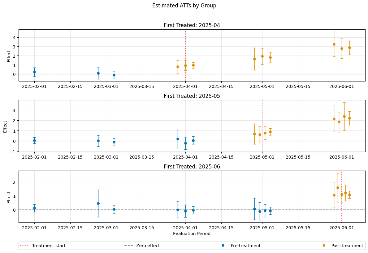
Universal Base Period#
The option gt_combinations="universal" set \(t_\text{pre} = \mathrm{g} - \delta - 1\), corresponding to a universal/constant comparison or base period.
Remark that this implies \(t_\text{pre} > t_\text{eval}\) for all pre-treatment periods (accounting for anticipation). Therefore these effects do not have the same straightforward interpretation as ATT’s.
[35]:
dml_obj_universal = DoubleMLDIDMulti(dml_data, **(default_args| {"gt_combinations": "universal"}))
dml_obj_universal.fit()
dml_obj_universal.bootstrap(n_rep_boot=5000)
dml_obj_universal.plot_effects()
/opt/hostedtoolcache/Python/3.12.13/x64/lib/python3.12/site-packages/sklearn/utils/validation.py:2739: UserWarning: X does not have valid feature names, but LGBMRegressor was fitted with feature names
  warnings.warn(
/opt/hostedtoolcache/Python/3.12.13/x64/lib/python3.12/site-packages/sklearn/utils/validation.py:2739: UserWarning: X does not have valid feature names, but LGBMRegressor was fitted with feature names
  warnings.warn(
/opt/hostedtoolcache/Python/3.12.13/x64/lib/python3.12/site-packages/sklearn/utils/validation.py:2739: UserWarning: X does not have valid feature names, but LGBMRegressor was fitted with feature names
  warnings.warn(
/opt/hostedtoolcache/Python/3.12.13/x64/lib/python3.12/site-packages/sklearn/utils/validation.py:2739: UserWarning: X does not have valid feature names, but LGBMRegressor was fitted with feature names
  warnings.warn(
/opt/hostedtoolcache/Python/3.12.13/x64/lib/python3.12/site-packages/sklearn/utils/validation.py:2739: UserWarning: X does not have valid feature names, but LGBMRegressor was fitted with feature names
  warnings.warn(
/opt/hostedtoolcache/Python/3.12.13/x64/lib/python3.12/site-packages/sklearn/utils/validation.py:2739: UserWarning: X does not have valid feature names, but LGBMRegressor was fitted with feature names
  warnings.warn(
/opt/hostedtoolcache/Python/3.12.13/x64/lib/python3.12/site-packages/sklearn/utils/validation.py:2739: UserWarning: X does not have valid feature names, but LGBMRegressor was fitted with feature names
  warnings.warn(
/opt/hostedtoolcache/Python/3.12.13/x64/lib/python3.12/site-packages/sklearn/utils/validation.py:2739: UserWarning: X does not have valid feature names, but LGBMRegressor was fitted with feature names
  warnings.warn(
/opt/hostedtoolcache/Python/3.12.13/x64/lib/python3.12/site-packages/sklearn/utils/validation.py:2739: UserWarning: X does not have valid feature names, but LGBMRegressor was fitted with feature names
  warnings.warn(
/opt/hostedtoolcache/Python/3.12.13/x64/lib/python3.12/site-packages/sklearn/utils/validation.py:2739: UserWarning: X does not have valid feature names, but LGBMRegressor was fitted with feature names
  warnings.warn(
/opt/hostedtoolcache/Python/3.12.13/x64/lib/python3.12/site-packages/sklearn/utils/validation.py:2739: UserWarning: X does not have valid feature names, but LGBMClassifier was fitted with feature names
  warnings.warn(
/opt/hostedtoolcache/Python/3.12.13/x64/lib/python3.12/site-packages/sklearn/utils/validation.py:2739: UserWarning: X does not have valid feature names, but LGBMClassifier was fitted with feature names
  warnings.warn(
/opt/hostedtoolcache/Python/3.12.13/x64/lib/python3.12/site-packages/sklearn/utils/validation.py:2739: UserWarning: X does not have valid feature names, but LGBMClassifier was fitted with feature names
  warnings.warn(
/opt/hostedtoolcache/Python/3.12.13/x64/lib/python3.12/site-packages/sklearn/utils/validation.py:2739: UserWarning: X does not have valid feature names, but LGBMClassifier was fitted with feature names
  warnings.warn(
/opt/hostedtoolcache/Python/3.12.13/x64/lib/python3.12/site-packages/sklearn/utils/validation.py:2739: UserWarning: X does not have valid feature names, but LGBMClassifier was fitted with feature names
  warnings.warn(
/opt/hostedtoolcache/Python/3.12.13/x64/lib/python3.12/site-packages/sklearn/utils/validation.py:2739: UserWarning: X does not have valid feature names, but LGBMRegressor was fitted with feature names
  warnings.warn(
/opt/hostedtoolcache/Python/3.12.13/x64/lib/python3.12/site-packages/sklearn/utils/validation.py:2739: UserWarning: X does not have valid feature names, but LGBMRegressor was fitted with feature names
  warnings.warn(
/opt/hostedtoolcache/Python/3.12.13/x64/lib/python3.12/site-packages/sklearn/utils/validation.py:2739: UserWarning: X does not have valid feature names, but LGBMRegressor was fitted with feature names
  warnings.warn(
/opt/hostedtoolcache/Python/3.12.13/x64/lib/python3.12/site-packages/sklearn/utils/validation.py:2739: UserWarning: X does not have valid feature names, but LGBMRegressor was fitted with feature names
  warnings.warn(
/opt/hostedtoolcache/Python/3.12.13/x64/lib/python3.12/site-packages/sklearn/utils/validation.py:2739: UserWarning: X does not have valid feature names, but LGBMRegressor was fitted with feature names
  warnings.warn(
/opt/hostedtoolcache/Python/3.12.13/x64/lib/python3.12/site-packages/sklearn/utils/validation.py:2739: UserWarning: X does not have valid feature names, but LGBMRegressor was fitted with feature names
  warnings.warn(
/opt/hostedtoolcache/Python/3.12.13/x64/lib/python3.12/site-packages/sklearn/utils/validation.py:2739: UserWarning: X does not have valid feature names, but LGBMRegressor was fitted with feature names
  warnings.warn(
/opt/hostedtoolcache/Python/3.12.13/x64/lib/python3.12/site-packages/sklearn/utils/validation.py:2739: UserWarning: X does not have valid feature names, but LGBMRegressor was fitted with feature names
  warnings.warn(
/opt/hostedtoolcache/Python/3.12.13/x64/lib/python3.12/site-packages/sklearn/utils/validation.py:2739: UserWarning: X does not have valid feature names, but LGBMRegressor was fitted with feature names
  warnings.warn(
/opt/hostedtoolcache/Python/3.12.13/x64/lib/python3.12/site-packages/sklearn/utils/validation.py:2739: UserWarning: X does not have valid feature names, but LGBMRegressor was fitted with feature names
  warnings.warn(
/opt/hostedtoolcache/Python/3.12.13/x64/lib/python3.12/site-packages/sklearn/utils/validation.py:2739: UserWarning: X does not have valid feature names, but LGBMClassifier was fitted with feature names
  warnings.warn(
/opt/hostedtoolcache/Python/3.12.13/x64/lib/python3.12/site-packages/sklearn/utils/validation.py:2739: UserWarning: X does not have valid feature names, but LGBMClassifier was fitted with feature names
  warnings.warn(
/opt/hostedtoolcache/Python/3.12.13/x64/lib/python3.12/site-packages/sklearn/utils/validation.py:2739: UserWarning: X does not have valid feature names, but LGBMClassifier was fitted with feature names
  warnings.warn(
/opt/hostedtoolcache/Python/3.12.13/x64/lib/python3.12/site-packages/sklearn/utils/validation.py:2739: UserWarning: X does not have valid feature names, but LGBMClassifier was fitted with feature names
  warnings.warn(
/opt/hostedtoolcache/Python/3.12.13/x64/lib/python3.12/site-packages/sklearn/utils/validation.py:2739: UserWarning: X does not have valid feature names, but LGBMClassifier was fitted with feature names
  warnings.warn(
/opt/hostedtoolcache/Python/3.12.13/x64/lib/python3.12/site-packages/sklearn/utils/validation.py:2739: UserWarning: X does not have valid feature names, but LGBMRegressor was fitted with feature names
  warnings.warn(
/opt/hostedtoolcache/Python/3.12.13/x64/lib/python3.12/site-packages/sklearn/utils/validation.py:2739: UserWarning: X does not have valid feature names, but LGBMRegressor was fitted with feature names
  warnings.warn(
/opt/hostedtoolcache/Python/3.12.13/x64/lib/python3.12/site-packages/sklearn/utils/validation.py:2739: UserWarning: X does not have valid feature names, but LGBMRegressor was fitted with feature names
  warnings.warn(
/opt/hostedtoolcache/Python/3.12.13/x64/lib/python3.12/site-packages/sklearn/utils/validation.py:2739: UserWarning: X does not have valid feature names, but LGBMRegressor was fitted with feature names
  warnings.warn(
/opt/hostedtoolcache/Python/3.12.13/x64/lib/python3.12/site-packages/sklearn/utils/validation.py:2739: UserWarning: X does not have valid feature names, but LGBMRegressor was fitted with feature names
  warnings.warn(
/opt/hostedtoolcache/Python/3.12.13/x64/lib/python3.12/site-packages/sklearn/utils/validation.py:2739: UserWarning: X does not have valid feature names, but LGBMRegressor was fitted with feature names
  warnings.warn(
/opt/hostedtoolcache/Python/3.12.13/x64/lib/python3.12/site-packages/sklearn/utils/validation.py:2739: UserWarning: X does not have valid feature names, but LGBMRegressor was fitted with feature names
  warnings.warn(
/opt/hostedtoolcache/Python/3.12.13/x64/lib/python3.12/site-packages/sklearn/utils/validation.py:2739: UserWarning: X does not have valid feature names, but LGBMRegressor was fitted with feature names
  warnings.warn(
/opt/hostedtoolcache/Python/3.12.13/x64/lib/python3.12/site-packages/sklearn/utils/validation.py:2739: UserWarning: X does not have valid feature names, but LGBMRegressor was fitted with feature names
  warnings.warn(
/opt/hostedtoolcache/Python/3.12.13/x64/lib/python3.12/site-packages/sklearn/utils/validation.py:2739: UserWarning: X does not have valid feature names, but LGBMRegressor was fitted with feature names
  warnings.warn(
/opt/hostedtoolcache/Python/3.12.13/x64/lib/python3.12/site-packages/sklearn/utils/validation.py:2739: UserWarning: X does not have valid feature names, but LGBMClassifier was fitted with feature names
  warnings.warn(
/opt/hostedtoolcache/Python/3.12.13/x64/lib/python3.12/site-packages/sklearn/utils/validation.py:2739: UserWarning: X does not have valid feature names, but LGBMClassifier was fitted with feature names
  warnings.warn(
/opt/hostedtoolcache/Python/3.12.13/x64/lib/python3.12/site-packages/sklearn/utils/validation.py:2739: UserWarning: X does not have valid feature names, but LGBMClassifier was fitted with feature names
  warnings.warn(
/opt/hostedtoolcache/Python/3.12.13/x64/lib/python3.12/site-packages/sklearn/utils/validation.py:2739: UserWarning: X does not have valid feature names, but LGBMClassifier was fitted with feature names
  warnings.warn(
/opt/hostedtoolcache/Python/3.12.13/x64/lib/python3.12/site-packages/sklearn/utils/validation.py:2739: UserWarning: X does not have valid feature names, but LGBMClassifier was fitted with feature names
  warnings.warn(
/opt/hostedtoolcache/Python/3.12.13/x64/lib/python3.12/site-packages/sklearn/utils/validation.py:2739: UserWarning: X does not have valid feature names, but LGBMRegressor was fitted with feature names
  warnings.warn(
/opt/hostedtoolcache/Python/3.12.13/x64/lib/python3.12/site-packages/sklearn/utils/validation.py:2739: UserWarning: X does not have valid feature names, but LGBMRegressor was fitted with feature names
  warnings.warn(
/opt/hostedtoolcache/Python/3.12.13/x64/lib/python3.12/site-packages/sklearn/utils/validation.py:2739: UserWarning: X does not have valid feature names, but LGBMRegressor was fitted with feature names
  warnings.warn(
/opt/hostedtoolcache/Python/3.12.13/x64/lib/python3.12/site-packages/sklearn/utils/validation.py:2739: UserWarning: X does not have valid feature names, but LGBMRegressor was fitted with feature names
  warnings.warn(
/opt/hostedtoolcache/Python/3.12.13/x64/lib/python3.12/site-packages/sklearn/utils/validation.py:2739: UserWarning: X does not have valid feature names, but LGBMRegressor was fitted with feature names
  warnings.warn(
/opt/hostedtoolcache/Python/3.12.13/x64/lib/python3.12/site-packages/sklearn/utils/validation.py:2739: UserWarning: X does not have valid feature names, but LGBMRegressor was fitted with feature names
  warnings.warn(
/opt/hostedtoolcache/Python/3.12.13/x64/lib/python3.12/site-packages/sklearn/utils/validation.py:2739: UserWarning: X does not have valid feature names, but LGBMRegressor was fitted with feature names
  warnings.warn(
/opt/hostedtoolcache/Python/3.12.13/x64/lib/python3.12/site-packages/sklearn/utils/validation.py:2739: UserWarning: X does not have valid feature names, but LGBMRegressor was fitted with feature names
  warnings.warn(
/opt/hostedtoolcache/Python/3.12.13/x64/lib/python3.12/site-packages/sklearn/utils/validation.py:2739: UserWarning: X does not have valid feature names, but LGBMRegressor was fitted with feature names
  warnings.warn(
/opt/hostedtoolcache/Python/3.12.13/x64/lib/python3.12/site-packages/sklearn/utils/validation.py:2739: UserWarning: X does not have valid feature names, but LGBMRegressor was fitted with feature names
  warnings.warn(
/opt/hostedtoolcache/Python/3.12.13/x64/lib/python3.12/site-packages/sklearn/utils/validation.py:2739: UserWarning: X does not have valid feature names, but LGBMClassifier was fitted with feature names
  warnings.warn(
/opt/hostedtoolcache/Python/3.12.13/x64/lib/python3.12/site-packages/sklearn/utils/validation.py:2739: UserWarning: X does not have valid feature names, but LGBMClassifier was fitted with feature names
  warnings.warn(
/opt/hostedtoolcache/Python/3.12.13/x64/lib/python3.12/site-packages/sklearn/utils/validation.py:2739: UserWarning: X does not have valid feature names, but LGBMClassifier was fitted with feature names
  warnings.warn(
/opt/hostedtoolcache/Python/3.12.13/x64/lib/python3.12/site-packages/sklearn/utils/validation.py:2739: UserWarning: X does not have valid feature names, but LGBMClassifier was fitted with feature names
  warnings.warn(
/opt/hostedtoolcache/Python/3.12.13/x64/lib/python3.12/site-packages/sklearn/utils/validation.py:2739: UserWarning: X does not have valid feature names, but LGBMClassifier was fitted with feature names
  warnings.warn(
/opt/hostedtoolcache/Python/3.12.13/x64/lib/python3.12/site-packages/sklearn/utils/validation.py:2739: UserWarning: X does not have valid feature names, but LGBMRegressor was fitted with feature names
  warnings.warn(
/opt/hostedtoolcache/Python/3.12.13/x64/lib/python3.12/site-packages/sklearn/utils/validation.py:2739: UserWarning: X does not have valid feature names, but LGBMRegressor was fitted with feature names
  warnings.warn(
/opt/hostedtoolcache/Python/3.12.13/x64/lib/python3.12/site-packages/sklearn/utils/validation.py:2739: UserWarning: X does not have valid feature names, but LGBMRegressor was fitted with feature names
  warnings.warn(
/opt/hostedtoolcache/Python/3.12.13/x64/lib/python3.12/site-packages/sklearn/utils/validation.py:2739: UserWarning: X does not have valid feature names, but LGBMRegressor was fitted with feature names
  warnings.warn(
/opt/hostedtoolcache/Python/3.12.13/x64/lib/python3.12/site-packages/sklearn/utils/validation.py:2739: UserWarning: X does not have valid feature names, but LGBMRegressor was fitted with feature names
  warnings.warn(
/opt/hostedtoolcache/Python/3.12.13/x64/lib/python3.12/site-packages/sklearn/utils/validation.py:2739: UserWarning: X does not have valid feature names, but LGBMRegressor was fitted with feature names
  warnings.warn(
/opt/hostedtoolcache/Python/3.12.13/x64/lib/python3.12/site-packages/sklearn/utils/validation.py:2739: UserWarning: X does not have valid feature names, but LGBMRegressor was fitted with feature names
  warnings.warn(
/opt/hostedtoolcache/Python/3.12.13/x64/lib/python3.12/site-packages/sklearn/utils/validation.py:2739: UserWarning: X does not have valid feature names, but LGBMRegressor was fitted with feature names
  warnings.warn(
/opt/hostedtoolcache/Python/3.12.13/x64/lib/python3.12/site-packages/sklearn/utils/validation.py:2739: UserWarning: X does not have valid feature names, but LGBMRegressor was fitted with feature names
  warnings.warn(
/opt/hostedtoolcache/Python/3.12.13/x64/lib/python3.12/site-packages/sklearn/utils/validation.py:2739: UserWarning: X does not have valid feature names, but LGBMRegressor was fitted with feature names
  warnings.warn(
/opt/hostedtoolcache/Python/3.12.13/x64/lib/python3.12/site-packages/sklearn/utils/validation.py:2739: UserWarning: X does not have valid feature names, but LGBMClassifier was fitted with feature names
  warnings.warn(
/opt/hostedtoolcache/Python/3.12.13/x64/lib/python3.12/site-packages/sklearn/utils/validation.py:2739: UserWarning: X does not have valid feature names, but LGBMClassifier was fitted with feature names
  warnings.warn(
/opt/hostedtoolcache/Python/3.12.13/x64/lib/python3.12/site-packages/sklearn/utils/validation.py:2739: UserWarning: X does not have valid feature names, but LGBMClassifier was fitted with feature names
  warnings.warn(
/opt/hostedtoolcache/Python/3.12.13/x64/lib/python3.12/site-packages/sklearn/utils/validation.py:2739: UserWarning: X does not have valid feature names, but LGBMClassifier was fitted with feature names
  warnings.warn(
/opt/hostedtoolcache/Python/3.12.13/x64/lib/python3.12/site-packages/sklearn/utils/validation.py:2739: UserWarning: X does not have valid feature names, but LGBMClassifier was fitted with feature names
  warnings.warn(
/opt/hostedtoolcache/Python/3.12.13/x64/lib/python3.12/site-packages/sklearn/utils/validation.py:2739: UserWarning: X does not have valid feature names, but LGBMRegressor was fitted with feature names
  warnings.warn(
/opt/hostedtoolcache/Python/3.12.13/x64/lib/python3.12/site-packages/sklearn/utils/validation.py:2739: UserWarning: X does not have valid feature names, but LGBMRegressor was fitted with feature names
  warnings.warn(
/opt/hostedtoolcache/Python/3.12.13/x64/lib/python3.12/site-packages/sklearn/utils/validation.py:2739: UserWarning: X does not have valid feature names, but LGBMRegressor was fitted with feature names
  warnings.warn(
/opt/hostedtoolcache/Python/3.12.13/x64/lib/python3.12/site-packages/sklearn/utils/validation.py:2739: UserWarning: X does not have valid feature names, but LGBMRegressor was fitted with feature names
  warnings.warn(
/opt/hostedtoolcache/Python/3.12.13/x64/lib/python3.12/site-packages/sklearn/utils/validation.py:2739: UserWarning: X does not have valid feature names, but LGBMRegressor was fitted with feature names
  warnings.warn(
/opt/hostedtoolcache/Python/3.12.13/x64/lib/python3.12/site-packages/sklearn/utils/validation.py:2739: UserWarning: X does not have valid feature names, but LGBMRegressor was fitted with feature names
  warnings.warn(
/opt/hostedtoolcache/Python/3.12.13/x64/lib/python3.12/site-packages/sklearn/utils/validation.py:2739: UserWarning: X does not have valid feature names, but LGBMRegressor was fitted with feature names
  warnings.warn(
/opt/hostedtoolcache/Python/3.12.13/x64/lib/python3.12/site-packages/sklearn/utils/validation.py:2739: UserWarning: X does not have valid feature names, but LGBMRegressor was fitted with feature names
  warnings.warn(
/opt/hostedtoolcache/Python/3.12.13/x64/lib/python3.12/site-packages/sklearn/utils/validation.py:2739: UserWarning: X does not have valid feature names, but LGBMRegressor was fitted with feature names
  warnings.warn(
/opt/hostedtoolcache/Python/3.12.13/x64/lib/python3.12/site-packages/sklearn/utils/validation.py:2739: UserWarning: X does not have valid feature names, but LGBMRegressor was fitted with feature names
  warnings.warn(
/opt/hostedtoolcache/Python/3.12.13/x64/lib/python3.12/site-packages/sklearn/utils/validation.py:2739: UserWarning: X does not have valid feature names, but LGBMClassifier was fitted with feature names
  warnings.warn(
/opt/hostedtoolcache/Python/3.12.13/x64/lib/python3.12/site-packages/sklearn/utils/validation.py:2739: UserWarning: X does not have valid feature names, but LGBMClassifier was fitted with feature names
  warnings.warn(
/opt/hostedtoolcache/Python/3.12.13/x64/lib/python3.12/site-packages/sklearn/utils/validation.py:2739: UserWarning: X does not have valid feature names, but LGBMClassifier was fitted with feature names
  warnings.warn(
/opt/hostedtoolcache/Python/3.12.13/x64/lib/python3.12/site-packages/sklearn/utils/validation.py:2739: UserWarning: X does not have valid feature names, but LGBMClassifier was fitted with feature names
  warnings.warn(
/opt/hostedtoolcache/Python/3.12.13/x64/lib/python3.12/site-packages/sklearn/utils/validation.py:2739: UserWarning: X does not have valid feature names, but LGBMClassifier was fitted with feature names
  warnings.warn(
/opt/hostedtoolcache/Python/3.12.13/x64/lib/python3.12/site-packages/sklearn/utils/validation.py:2739: UserWarning: X does not have valid feature names, but LGBMRegressor was fitted with feature names
  warnings.warn(
/opt/hostedtoolcache/Python/3.12.13/x64/lib/python3.12/site-packages/sklearn/utils/validation.py:2739: UserWarning: X does not have valid feature names, but LGBMRegressor was fitted with feature names
  warnings.warn(
/opt/hostedtoolcache/Python/3.12.13/x64/lib/python3.12/site-packages/sklearn/utils/validation.py:2739: UserWarning: X does not have valid feature names, but LGBMRegressor was fitted with feature names
  warnings.warn(
/opt/hostedtoolcache/Python/3.12.13/x64/lib/python3.12/site-packages/sklearn/utils/validation.py:2739: UserWarning: X does not have valid feature names, but LGBMRegressor was fitted with feature names
  warnings.warn(
/opt/hostedtoolcache/Python/3.12.13/x64/lib/python3.12/site-packages/sklearn/utils/validation.py:2739: UserWarning: X does not have valid feature names, but LGBMRegressor was fitted with feature names
  warnings.warn(
/opt/hostedtoolcache/Python/3.12.13/x64/lib/python3.12/site-packages/sklearn/utils/validation.py:2739: UserWarning: X does not have valid feature names, but LGBMRegressor was fitted with feature names
  warnings.warn(
/opt/hostedtoolcache/Python/3.12.13/x64/lib/python3.12/site-packages/sklearn/utils/validation.py:2739: UserWarning: X does not have valid feature names, but LGBMRegressor was fitted with feature names
  warnings.warn(
/opt/hostedtoolcache/Python/3.12.13/x64/lib/python3.12/site-packages/sklearn/utils/validation.py:2739: UserWarning: X does not have valid feature names, but LGBMRegressor was fitted with feature names
  warnings.warn(
/opt/hostedtoolcache/Python/3.12.13/x64/lib/python3.12/site-packages/sklearn/utils/validation.py:2739: UserWarning: X does not have valid feature names, but LGBMRegressor was fitted with feature names
  warnings.warn(
/opt/hostedtoolcache/Python/3.12.13/x64/lib/python3.12/site-packages/sklearn/utils/validation.py:2739: UserWarning: X does not have valid feature names, but LGBMRegressor was fitted with feature names
  warnings.warn(
/opt/hostedtoolcache/Python/3.12.13/x64/lib/python3.12/site-packages/sklearn/utils/validation.py:2739: UserWarning: X does not have valid feature names, but LGBMClassifier was fitted with feature names
  warnings.warn(
/opt/hostedtoolcache/Python/3.12.13/x64/lib/python3.12/site-packages/sklearn/utils/validation.py:2739: UserWarning: X does not have valid feature names, but LGBMClassifier was fitted with feature names
  warnings.warn(
/opt/hostedtoolcache/Python/3.12.13/x64/lib/python3.12/site-packages/sklearn/utils/validation.py:2739: UserWarning: X does not have valid feature names, but LGBMClassifier was fitted with feature names
  warnings.warn(
/opt/hostedtoolcache/Python/3.12.13/x64/lib/python3.12/site-packages/sklearn/utils/validation.py:2739: UserWarning: X does not have valid feature names, but LGBMClassifier was fitted with feature names
  warnings.warn(
/opt/hostedtoolcache/Python/3.12.13/x64/lib/python3.12/site-packages/sklearn/utils/validation.py:2739: UserWarning: X does not have valid feature names, but LGBMClassifier was fitted with feature names
  warnings.warn(
/opt/hostedtoolcache/Python/3.12.13/x64/lib/python3.12/site-packages/sklearn/utils/validation.py:2739: UserWarning: X does not have valid feature names, but LGBMRegressor was fitted with feature names
  warnings.warn(
/opt/hostedtoolcache/Python/3.12.13/x64/lib/python3.12/site-packages/sklearn/utils/validation.py:2739: UserWarning: X does not have valid feature names, but LGBMRegressor was fitted with feature names
  warnings.warn(
/opt/hostedtoolcache/Python/3.12.13/x64/lib/python3.12/site-packages/sklearn/utils/validation.py:2739: UserWarning: X does not have valid feature names, but LGBMRegressor was fitted with feature names
  warnings.warn(
/opt/hostedtoolcache/Python/3.12.13/x64/lib/python3.12/site-packages/sklearn/utils/validation.py:2739: UserWarning: X does not have valid feature names, but LGBMRegressor was fitted with feature names
  warnings.warn(
/opt/hostedtoolcache/Python/3.12.13/x64/lib/python3.12/site-packages/sklearn/utils/validation.py:2739: UserWarning: X does not have valid feature names, but LGBMRegressor was fitted with feature names
  warnings.warn(
/opt/hostedtoolcache/Python/3.12.13/x64/lib/python3.12/site-packages/sklearn/utils/validation.py:2739: UserWarning: X does not have valid feature names, but LGBMRegressor was fitted with feature names
  warnings.warn(
/opt/hostedtoolcache/Python/3.12.13/x64/lib/python3.12/site-packages/sklearn/utils/validation.py:2739: UserWarning: X does not have valid feature names, but LGBMRegressor was fitted with feature names
  warnings.warn(
/opt/hostedtoolcache/Python/3.12.13/x64/lib/python3.12/site-packages/sklearn/utils/validation.py:2739: UserWarning: X does not have valid feature names, but LGBMRegressor was fitted with feature names
  warnings.warn(
/opt/hostedtoolcache/Python/3.12.13/x64/lib/python3.12/site-packages/sklearn/utils/validation.py:2739: UserWarning: X does not have valid feature names, but LGBMRegressor was fitted with feature names
  warnings.warn(
/opt/hostedtoolcache/Python/3.12.13/x64/lib/python3.12/site-packages/sklearn/utils/validation.py:2739: UserWarning: X does not have valid feature names, but LGBMRegressor was fitted with feature names
  warnings.warn(
/opt/hostedtoolcache/Python/3.12.13/x64/lib/python3.12/site-packages/sklearn/utils/validation.py:2739: UserWarning: X does not have valid feature names, but LGBMClassifier was fitted with feature names
  warnings.warn(
/opt/hostedtoolcache/Python/3.12.13/x64/lib/python3.12/site-packages/sklearn/utils/validation.py:2739: UserWarning: X does not have valid feature names, but LGBMClassifier was fitted with feature names
  warnings.warn(
/opt/hostedtoolcache/Python/3.12.13/x64/lib/python3.12/site-packages/sklearn/utils/validation.py:2739: UserWarning: X does not have valid feature names, but LGBMClassifier was fitted with feature names
  warnings.warn(
/opt/hostedtoolcache/Python/3.12.13/x64/lib/python3.12/site-packages/sklearn/utils/validation.py:2739: UserWarning: X does not have valid feature names, but LGBMClassifier was fitted with feature names
  warnings.warn(
/opt/hostedtoolcache/Python/3.12.13/x64/lib/python3.12/site-packages/sklearn/utils/validation.py:2739: UserWarning: X does not have valid feature names, but LGBMClassifier was fitted with feature names
  warnings.warn(
/opt/hostedtoolcache/Python/3.12.13/x64/lib/python3.12/site-packages/sklearn/utils/validation.py:2739: UserWarning: X does not have valid feature names, but LGBMRegressor was fitted with feature names
  warnings.warn(
/opt/hostedtoolcache/Python/3.12.13/x64/lib/python3.12/site-packages/sklearn/utils/validation.py:2739: UserWarning: X does not have valid feature names, but LGBMRegressor was fitted with feature names
  warnings.warn(
/opt/hostedtoolcache/Python/3.12.13/x64/lib/python3.12/site-packages/sklearn/utils/validation.py:2739: UserWarning: X does not have valid feature names, but LGBMRegressor was fitted with feature names
  warnings.warn(
/opt/hostedtoolcache/Python/3.12.13/x64/lib/python3.12/site-packages/sklearn/utils/validation.py:2739: UserWarning: X does not have valid feature names, but LGBMRegressor was fitted with feature names
  warnings.warn(
/opt/hostedtoolcache/Python/3.12.13/x64/lib/python3.12/site-packages/sklearn/utils/validation.py:2739: UserWarning: X does not have valid feature names, but LGBMRegressor was fitted with feature names
  warnings.warn(
/opt/hostedtoolcache/Python/3.12.13/x64/lib/python3.12/site-packages/sklearn/utils/validation.py:2739: UserWarning: X does not have valid feature names, but LGBMRegressor was fitted with feature names
  warnings.warn(
/opt/hostedtoolcache/Python/3.12.13/x64/lib/python3.12/site-packages/sklearn/utils/validation.py:2739: UserWarning: X does not have valid feature names, but LGBMRegressor was fitted with feature names
  warnings.warn(
/opt/hostedtoolcache/Python/3.12.13/x64/lib/python3.12/site-packages/sklearn/utils/validation.py:2739: UserWarning: X does not have valid feature names, but LGBMRegressor was fitted with feature names
  warnings.warn(
/opt/hostedtoolcache/Python/3.12.13/x64/lib/python3.12/site-packages/sklearn/utils/validation.py:2739: UserWarning: X does not have valid feature names, but LGBMRegressor was fitted with feature names
  warnings.warn(
/opt/hostedtoolcache/Python/3.12.13/x64/lib/python3.12/site-packages/sklearn/utils/validation.py:2739: UserWarning: X does not have valid feature names, but LGBMRegressor was fitted with feature names
  warnings.warn(
/opt/hostedtoolcache/Python/3.12.13/x64/lib/python3.12/site-packages/sklearn/utils/validation.py:2739: UserWarning: X does not have valid feature names, but LGBMClassifier was fitted with feature names
  warnings.warn(
/opt/hostedtoolcache/Python/3.12.13/x64/lib/python3.12/site-packages/sklearn/utils/validation.py:2739: UserWarning: X does not have valid feature names, but LGBMClassifier was fitted with feature names
  warnings.warn(
/opt/hostedtoolcache/Python/3.12.13/x64/lib/python3.12/site-packages/sklearn/utils/validation.py:2739: UserWarning: X does not have valid feature names, but LGBMClassifier was fitted with feature names
  warnings.warn(
/opt/hostedtoolcache/Python/3.12.13/x64/lib/python3.12/site-packages/sklearn/utils/validation.py:2739: UserWarning: X does not have valid feature names, but LGBMClassifier was fitted with feature names
  warnings.warn(
/opt/hostedtoolcache/Python/3.12.13/x64/lib/python3.12/site-packages/sklearn/utils/validation.py:2739: UserWarning: X does not have valid feature names, but LGBMClassifier was fitted with feature names
  warnings.warn(
/opt/hostedtoolcache/Python/3.12.13/x64/lib/python3.12/site-packages/sklearn/utils/validation.py:2739: UserWarning: X does not have valid feature names, but LGBMRegressor was fitted with feature names
  warnings.warn(
/opt/hostedtoolcache/Python/3.12.13/x64/lib/python3.12/site-packages/sklearn/utils/validation.py:2739: UserWarning: X does not have valid feature names, but LGBMRegressor was fitted with feature names
  warnings.warn(
/opt/hostedtoolcache/Python/3.12.13/x64/lib/python3.12/site-packages/sklearn/utils/validation.py:2739: UserWarning: X does not have valid feature names, but LGBMRegressor was fitted with feature names
  warnings.warn(
/opt/hostedtoolcache/Python/3.12.13/x64/lib/python3.12/site-packages/sklearn/utils/validation.py:2739: UserWarning: X does not have valid feature names, but LGBMRegressor was fitted with feature names
  warnings.warn(
/opt/hostedtoolcache/Python/3.12.13/x64/lib/python3.12/site-packages/sklearn/utils/validation.py:2739: UserWarning: X does not have valid feature names, but LGBMRegressor was fitted with feature names
  warnings.warn(
/opt/hostedtoolcache/Python/3.12.13/x64/lib/python3.12/site-packages/sklearn/utils/validation.py:2739: UserWarning: X does not have valid feature names, but LGBMRegressor was fitted with feature names
  warnings.warn(
/opt/hostedtoolcache/Python/3.12.13/x64/lib/python3.12/site-packages/sklearn/utils/validation.py:2739: UserWarning: X does not have valid feature names, but LGBMRegressor was fitted with feature names
  warnings.warn(
/opt/hostedtoolcache/Python/3.12.13/x64/lib/python3.12/site-packages/sklearn/utils/validation.py:2739: UserWarning: X does not have valid feature names, but LGBMRegressor was fitted with feature names
  warnings.warn(
/opt/hostedtoolcache/Python/3.12.13/x64/lib/python3.12/site-packages/sklearn/utils/validation.py:2739: UserWarning: X does not have valid feature names, but LGBMRegressor was fitted with feature names
  warnings.warn(
/opt/hostedtoolcache/Python/3.12.13/x64/lib/python3.12/site-packages/sklearn/utils/validation.py:2739: UserWarning: X does not have valid feature names, but LGBMRegressor was fitted with feature names
  warnings.warn(
/opt/hostedtoolcache/Python/3.12.13/x64/lib/python3.12/site-packages/sklearn/utils/validation.py:2739: UserWarning: X does not have valid feature names, but LGBMClassifier was fitted with feature names
  warnings.warn(
/opt/hostedtoolcache/Python/3.12.13/x64/lib/python3.12/site-packages/sklearn/utils/validation.py:2739: UserWarning: X does not have valid feature names, but LGBMClassifier was fitted with feature names
  warnings.warn(
/opt/hostedtoolcache/Python/3.12.13/x64/lib/python3.12/site-packages/sklearn/utils/validation.py:2739: UserWarning: X does not have valid feature names, but LGBMClassifier was fitted with feature names
  warnings.warn(
/opt/hostedtoolcache/Python/3.12.13/x64/lib/python3.12/site-packages/sklearn/utils/validation.py:2739: UserWarning: X does not have valid feature names, but LGBMClassifier was fitted with feature names
  warnings.warn(
/opt/hostedtoolcache/Python/3.12.13/x64/lib/python3.12/site-packages/sklearn/utils/validation.py:2739: UserWarning: X does not have valid feature names, but LGBMClassifier was fitted with feature names
  warnings.warn(
/opt/hostedtoolcache/Python/3.12.13/x64/lib/python3.12/site-packages/sklearn/utils/validation.py:2739: UserWarning: X does not have valid feature names, but LGBMRegressor was fitted with feature names
  warnings.warn(
/opt/hostedtoolcache/Python/3.12.13/x64/lib/python3.12/site-packages/sklearn/utils/validation.py:2739: UserWarning: X does not have valid feature names, but LGBMRegressor was fitted with feature names
  warnings.warn(
/opt/hostedtoolcache/Python/3.12.13/x64/lib/python3.12/site-packages/sklearn/utils/validation.py:2739: UserWarning: X does not have valid feature names, but LGBMRegressor was fitted with feature names
  warnings.warn(
/opt/hostedtoolcache/Python/3.12.13/x64/lib/python3.12/site-packages/sklearn/utils/validation.py:2739: UserWarning: X does not have valid feature names, but LGBMRegressor was fitted with feature names
  warnings.warn(
/opt/hostedtoolcache/Python/3.12.13/x64/lib/python3.12/site-packages/sklearn/utils/validation.py:2739: UserWarning: X does not have valid feature names, but LGBMRegressor was fitted with feature names
  warnings.warn(
/opt/hostedtoolcache/Python/3.12.13/x64/lib/python3.12/site-packages/sklearn/utils/validation.py:2739: UserWarning: X does not have valid feature names, but LGBMRegressor was fitted with feature names
  warnings.warn(
/opt/hostedtoolcache/Python/3.12.13/x64/lib/python3.12/site-packages/sklearn/utils/validation.py:2739: UserWarning: X does not have valid feature names, but LGBMRegressor was fitted with feature names
  warnings.warn(
/opt/hostedtoolcache/Python/3.12.13/x64/lib/python3.12/site-packages/sklearn/utils/validation.py:2739: UserWarning: X does not have valid feature names, but LGBMRegressor was fitted with feature names
  warnings.warn(
/opt/hostedtoolcache/Python/3.12.13/x64/lib/python3.12/site-packages/sklearn/utils/validation.py:2739: UserWarning: X does not have valid feature names, but LGBMRegressor was fitted with feature names
  warnings.warn(
/opt/hostedtoolcache/Python/3.12.13/x64/lib/python3.12/site-packages/sklearn/utils/validation.py:2739: UserWarning: X does not have valid feature names, but LGBMRegressor was fitted with feature names
  warnings.warn(
/opt/hostedtoolcache/Python/3.12.13/x64/lib/python3.12/site-packages/sklearn/utils/validation.py:2739: UserWarning: X does not have valid feature names, but LGBMClassifier was fitted with feature names
  warnings.warn(
/opt/hostedtoolcache/Python/3.12.13/x64/lib/python3.12/site-packages/sklearn/utils/validation.py:2739: UserWarning: X does not have valid feature names, but LGBMClassifier was fitted with feature names
  warnings.warn(
/opt/hostedtoolcache/Python/3.12.13/x64/lib/python3.12/site-packages/sklearn/utils/validation.py:2739: UserWarning: X does not have valid feature names, but LGBMClassifier was fitted with feature names
  warnings.warn(
/opt/hostedtoolcache/Python/3.12.13/x64/lib/python3.12/site-packages/sklearn/utils/validation.py:2739: UserWarning: X does not have valid feature names, but LGBMClassifier was fitted with feature names
  warnings.warn(
/opt/hostedtoolcache/Python/3.12.13/x64/lib/python3.12/site-packages/sklearn/utils/validation.py:2739: UserWarning: X does not have valid feature names, but LGBMClassifier was fitted with feature names
  warnings.warn(
/opt/hostedtoolcache/Python/3.12.13/x64/lib/python3.12/site-packages/sklearn/utils/validation.py:2739: UserWarning: X does not have valid feature names, but LGBMRegressor was fitted with feature names
  warnings.warn(
/opt/hostedtoolcache/Python/3.12.13/x64/lib/python3.12/site-packages/sklearn/utils/validation.py:2739: UserWarning: X does not have valid feature names, but LGBMRegressor was fitted with feature names
  warnings.warn(
/opt/hostedtoolcache/Python/3.12.13/x64/lib/python3.12/site-packages/sklearn/utils/validation.py:2739: UserWarning: X does not have valid feature names, but LGBMRegressor was fitted with feature names
  warnings.warn(
/opt/hostedtoolcache/Python/3.12.13/x64/lib/python3.12/site-packages/sklearn/utils/validation.py:2739: UserWarning: X does not have valid feature names, but LGBMRegressor was fitted with feature names
  warnings.warn(
/opt/hostedtoolcache/Python/3.12.13/x64/lib/python3.12/site-packages/sklearn/utils/validation.py:2739: UserWarning: X does not have valid feature names, but LGBMRegressor was fitted with feature names
  warnings.warn(
/opt/hostedtoolcache/Python/3.12.13/x64/lib/python3.12/site-packages/sklearn/utils/validation.py:2739: UserWarning: X does not have valid feature names, but LGBMRegressor was fitted with feature names
  warnings.warn(
/opt/hostedtoolcache/Python/3.12.13/x64/lib/python3.12/site-packages/sklearn/utils/validation.py:2739: UserWarning: X does not have valid feature names, but LGBMRegressor was fitted with feature names
  warnings.warn(
/opt/hostedtoolcache/Python/3.12.13/x64/lib/python3.12/site-packages/sklearn/utils/validation.py:2739: UserWarning: X does not have valid feature names, but LGBMRegressor was fitted with feature names
  warnings.warn(
/opt/hostedtoolcache/Python/3.12.13/x64/lib/python3.12/site-packages/sklearn/utils/validation.py:2739: UserWarning: X does not have valid feature names, but LGBMRegressor was fitted with feature names
  warnings.warn(
/opt/hostedtoolcache/Python/3.12.13/x64/lib/python3.12/site-packages/sklearn/utils/validation.py:2739: UserWarning: X does not have valid feature names, but LGBMRegressor was fitted with feature names
  warnings.warn(
/opt/hostedtoolcache/Python/3.12.13/x64/lib/python3.12/site-packages/sklearn/utils/validation.py:2739: UserWarning: X does not have valid feature names, but LGBMClassifier was fitted with feature names
  warnings.warn(
/opt/hostedtoolcache/Python/3.12.13/x64/lib/python3.12/site-packages/sklearn/utils/validation.py:2739: UserWarning: X does not have valid feature names, but LGBMClassifier was fitted with feature names
  warnings.warn(
/opt/hostedtoolcache/Python/3.12.13/x64/lib/python3.12/site-packages/sklearn/utils/validation.py:2739: UserWarning: X does not have valid feature names, but LGBMClassifier was fitted with feature names
  warnings.warn(
/opt/hostedtoolcache/Python/3.12.13/x64/lib/python3.12/site-packages/sklearn/utils/validation.py:2739: UserWarning: X does not have valid feature names, but LGBMClassifier was fitted with feature names
  warnings.warn(
/opt/hostedtoolcache/Python/3.12.13/x64/lib/python3.12/site-packages/sklearn/utils/validation.py:2739: UserWarning: X does not have valid feature names, but LGBMClassifier was fitted with feature names
  warnings.warn(
/opt/hostedtoolcache/Python/3.12.13/x64/lib/python3.12/site-packages/sklearn/utils/validation.py:2739: UserWarning: X does not have valid feature names, but LGBMRegressor was fitted with feature names
  warnings.warn(
/opt/hostedtoolcache/Python/3.12.13/x64/lib/python3.12/site-packages/sklearn/utils/validation.py:2739: UserWarning: X does not have valid feature names, but LGBMRegressor was fitted with feature names
  warnings.warn(
/opt/hostedtoolcache/Python/3.12.13/x64/lib/python3.12/site-packages/sklearn/utils/validation.py:2739: UserWarning: X does not have valid feature names, but LGBMRegressor was fitted with feature names
  warnings.warn(
/opt/hostedtoolcache/Python/3.12.13/x64/lib/python3.12/site-packages/sklearn/utils/validation.py:2739: UserWarning: X does not have valid feature names, but LGBMRegressor was fitted with feature names
  warnings.warn(
/opt/hostedtoolcache/Python/3.12.13/x64/lib/python3.12/site-packages/sklearn/utils/validation.py:2739: UserWarning: X does not have valid feature names, but LGBMRegressor was fitted with feature names
  warnings.warn(
/opt/hostedtoolcache/Python/3.12.13/x64/lib/python3.12/site-packages/sklearn/utils/validation.py:2739: UserWarning: X does not have valid feature names, but LGBMRegressor was fitted with feature names
  warnings.warn(
/opt/hostedtoolcache/Python/3.12.13/x64/lib/python3.12/site-packages/sklearn/utils/validation.py:2739: UserWarning: X does not have valid feature names, but LGBMRegressor was fitted with feature names
  warnings.warn(
/opt/hostedtoolcache/Python/3.12.13/x64/lib/python3.12/site-packages/sklearn/utils/validation.py:2739: UserWarning: X does not have valid feature names, but LGBMRegressor was fitted with feature names
  warnings.warn(
/opt/hostedtoolcache/Python/3.12.13/x64/lib/python3.12/site-packages/sklearn/utils/validation.py:2739: UserWarning: X does not have valid feature names, but LGBMRegressor was fitted with feature names
  warnings.warn(
/opt/hostedtoolcache/Python/3.12.13/x64/lib/python3.12/site-packages/sklearn/utils/validation.py:2739: UserWarning: X does not have valid feature names, but LGBMRegressor was fitted with feature names
  warnings.warn(
/opt/hostedtoolcache/Python/3.12.13/x64/lib/python3.12/site-packages/sklearn/utils/validation.py:2739: UserWarning: X does not have valid feature names, but LGBMClassifier was fitted with feature names
  warnings.warn(
/opt/hostedtoolcache/Python/3.12.13/x64/lib/python3.12/site-packages/sklearn/utils/validation.py:2739: UserWarning: X does not have valid feature names, but LGBMClassifier was fitted with feature names
  warnings.warn(
/opt/hostedtoolcache/Python/3.12.13/x64/lib/python3.12/site-packages/sklearn/utils/validation.py:2739: UserWarning: X does not have valid feature names, but LGBMClassifier was fitted with feature names
  warnings.warn(
/opt/hostedtoolcache/Python/3.12.13/x64/lib/python3.12/site-packages/sklearn/utils/validation.py:2739: UserWarning: X does not have valid feature names, but LGBMClassifier was fitted with feature names
  warnings.warn(
/opt/hostedtoolcache/Python/3.12.13/x64/lib/python3.12/site-packages/sklearn/utils/validation.py:2739: UserWarning: X does not have valid feature names, but LGBMClassifier was fitted with feature names
  warnings.warn(
/opt/hostedtoolcache/Python/3.12.13/x64/lib/python3.12/site-packages/sklearn/utils/validation.py:2739: UserWarning: X does not have valid feature names, but LGBMRegressor was fitted with feature names
  warnings.warn(
/opt/hostedtoolcache/Python/3.12.13/x64/lib/python3.12/site-packages/sklearn/utils/validation.py:2739: UserWarning: X does not have valid feature names, but LGBMRegressor was fitted with feature names
  warnings.warn(
/opt/hostedtoolcache/Python/3.12.13/x64/lib/python3.12/site-packages/sklearn/utils/validation.py:2739: UserWarning: X does not have valid feature names, but LGBMRegressor was fitted with feature names
  warnings.warn(
/opt/hostedtoolcache/Python/3.12.13/x64/lib/python3.12/site-packages/sklearn/utils/validation.py:2739: UserWarning: X does not have valid feature names, but LGBMRegressor was fitted with feature names
  warnings.warn(
/opt/hostedtoolcache/Python/3.12.13/x64/lib/python3.12/site-packages/sklearn/utils/validation.py:2739: UserWarning: X does not have valid feature names, but LGBMRegressor was fitted with feature names
  warnings.warn(
/opt/hostedtoolcache/Python/3.12.13/x64/lib/python3.12/site-packages/sklearn/utils/validation.py:2739: UserWarning: X does not have valid feature names, but LGBMRegressor was fitted with feature names
  warnings.warn(
/opt/hostedtoolcache/Python/3.12.13/x64/lib/python3.12/site-packages/sklearn/utils/validation.py:2739: UserWarning: X does not have valid feature names, but LGBMRegressor was fitted with feature names
  warnings.warn(
/opt/hostedtoolcache/Python/3.12.13/x64/lib/python3.12/site-packages/sklearn/utils/validation.py:2739: UserWarning: X does not have valid feature names, but LGBMRegressor was fitted with feature names
  warnings.warn(
/opt/hostedtoolcache/Python/3.12.13/x64/lib/python3.12/site-packages/sklearn/utils/validation.py:2739: UserWarning: X does not have valid feature names, but LGBMRegressor was fitted with feature names
  warnings.warn(
/opt/hostedtoolcache/Python/3.12.13/x64/lib/python3.12/site-packages/sklearn/utils/validation.py:2739: UserWarning: X does not have valid feature names, but LGBMRegressor was fitted with feature names
  warnings.warn(
/opt/hostedtoolcache/Python/3.12.13/x64/lib/python3.12/site-packages/sklearn/utils/validation.py:2739: UserWarning: X does not have valid feature names, but LGBMClassifier was fitted with feature names
  warnings.warn(
/opt/hostedtoolcache/Python/3.12.13/x64/lib/python3.12/site-packages/sklearn/utils/validation.py:2739: UserWarning: X does not have valid feature names, but LGBMClassifier was fitted with feature names
  warnings.warn(
/opt/hostedtoolcache/Python/3.12.13/x64/lib/python3.12/site-packages/sklearn/utils/validation.py:2739: UserWarning: X does not have valid feature names, but LGBMClassifier was fitted with feature names
  warnings.warn(
/opt/hostedtoolcache/Python/3.12.13/x64/lib/python3.12/site-packages/sklearn/utils/validation.py:2739: UserWarning: X does not have valid feature names, but LGBMClassifier was fitted with feature names
  warnings.warn(
/opt/hostedtoolcache/Python/3.12.13/x64/lib/python3.12/site-packages/sklearn/utils/validation.py:2739: UserWarning: X does not have valid feature names, but LGBMClassifier was fitted with feature names
  warnings.warn(
/opt/hostedtoolcache/Python/3.12.13/x64/lib/python3.12/site-packages/sklearn/utils/validation.py:2739: UserWarning: X does not have valid feature names, but LGBMRegressor was fitted with feature names
  warnings.warn(
/opt/hostedtoolcache/Python/3.12.13/x64/lib/python3.12/site-packages/sklearn/utils/validation.py:2739: UserWarning: X does not have valid feature names, but LGBMRegressor was fitted with feature names
  warnings.warn(
/opt/hostedtoolcache/Python/3.12.13/x64/lib/python3.12/site-packages/sklearn/utils/validation.py:2739: UserWarning: X does not have valid feature names, but LGBMRegressor was fitted with feature names
  warnings.warn(
/opt/hostedtoolcache/Python/3.12.13/x64/lib/python3.12/site-packages/sklearn/utils/validation.py:2739: UserWarning: X does not have valid feature names, but LGBMRegressor was fitted with feature names
  warnings.warn(
/opt/hostedtoolcache/Python/3.12.13/x64/lib/python3.12/site-packages/sklearn/utils/validation.py:2739: UserWarning: X does not have valid feature names, but LGBMRegressor was fitted with feature names
  warnings.warn(
/opt/hostedtoolcache/Python/3.12.13/x64/lib/python3.12/site-packages/sklearn/utils/validation.py:2739: UserWarning: X does not have valid feature names, but LGBMRegressor was fitted with feature names
  warnings.warn(
/opt/hostedtoolcache/Python/3.12.13/x64/lib/python3.12/site-packages/sklearn/utils/validation.py:2739: UserWarning: X does not have valid feature names, but LGBMRegressor was fitted with feature names
  warnings.warn(
/opt/hostedtoolcache/Python/3.12.13/x64/lib/python3.12/site-packages/sklearn/utils/validation.py:2739: UserWarning: X does not have valid feature names, but LGBMRegressor was fitted with feature names
  warnings.warn(
/opt/hostedtoolcache/Python/3.12.13/x64/lib/python3.12/site-packages/sklearn/utils/validation.py:2739: UserWarning: X does not have valid feature names, but LGBMRegressor was fitted with feature names
  warnings.warn(
/opt/hostedtoolcache/Python/3.12.13/x64/lib/python3.12/site-packages/sklearn/utils/validation.py:2739: UserWarning: X does not have valid feature names, but LGBMRegressor was fitted with feature names
  warnings.warn(
/opt/hostedtoolcache/Python/3.12.13/x64/lib/python3.12/site-packages/sklearn/utils/validation.py:2739: UserWarning: X does not have valid feature names, but LGBMClassifier was fitted with feature names
  warnings.warn(
/opt/hostedtoolcache/Python/3.12.13/x64/lib/python3.12/site-packages/sklearn/utils/validation.py:2739: UserWarning: X does not have valid feature names, but LGBMClassifier was fitted with feature names
  warnings.warn(
/opt/hostedtoolcache/Python/3.12.13/x64/lib/python3.12/site-packages/sklearn/utils/validation.py:2739: UserWarning: X does not have valid feature names, but LGBMClassifier was fitted with feature names
  warnings.warn(
/opt/hostedtoolcache/Python/3.12.13/x64/lib/python3.12/site-packages/sklearn/utils/validation.py:2739: UserWarning: X does not have valid feature names, but LGBMClassifier was fitted with feature names
  warnings.warn(
/opt/hostedtoolcache/Python/3.12.13/x64/lib/python3.12/site-packages/sklearn/utils/validation.py:2739: UserWarning: X does not have valid feature names, but LGBMClassifier was fitted with feature names
  warnings.warn(
[35]:
(<Figure size 1200x800 with 4 Axes>,
 [<Axes: title={'center': 'First Treated: 2025-04'}, ylabel='Effect'>,
  <Axes: title={'center': 'First Treated: 2025-05'}, ylabel='Effect'>,
  <Axes: title={'center': 'First Treated: 2025-06'}, xlabel='Evaluation Period', ylabel='Effect'>])
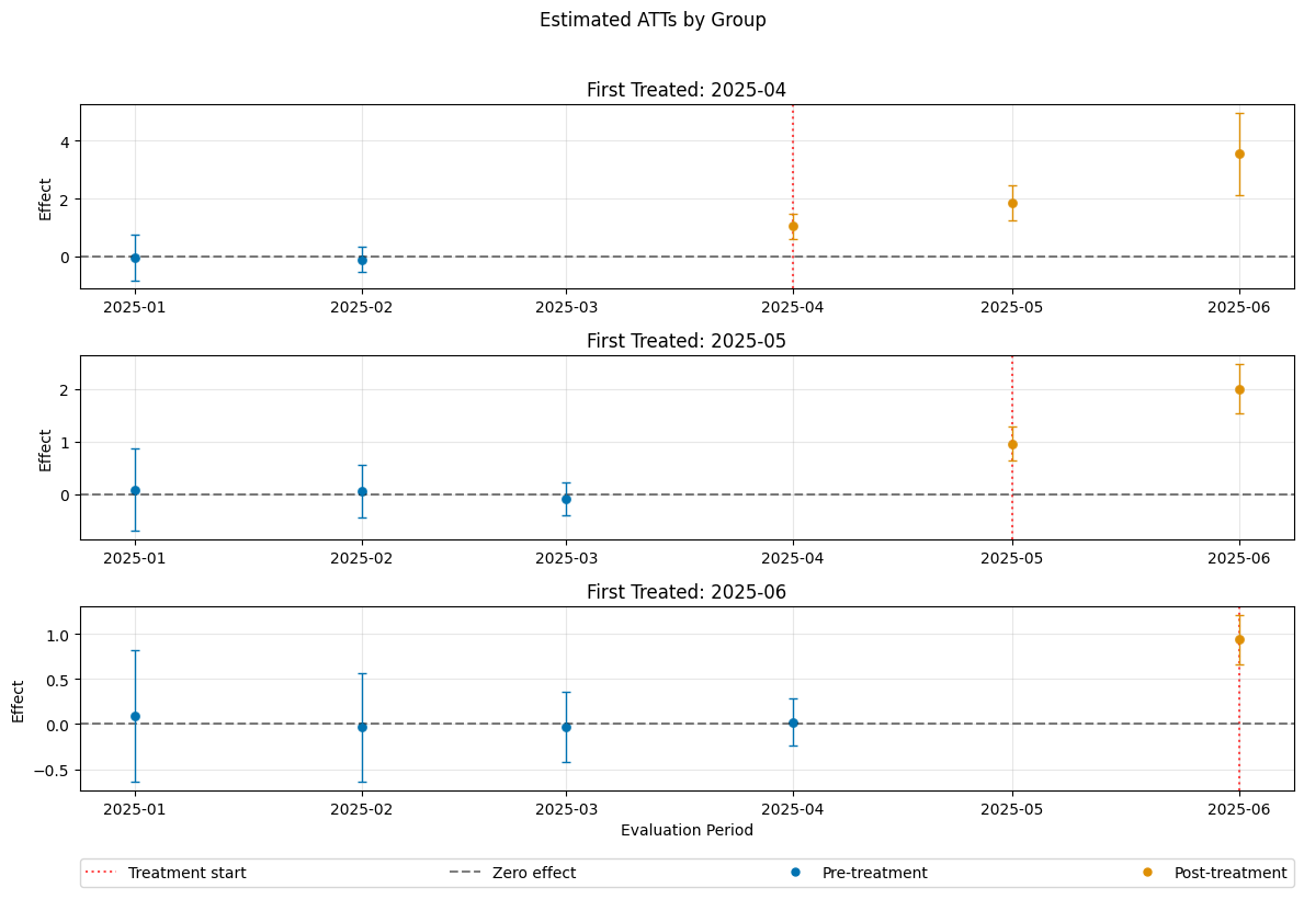
Selected Combinations#
Instead it is also possible to just submit a list of tuples containing \((\mathrm{g}, t_\text{pre}, t_\text{eval})\) combinations. E.g. only two combinations
[36]:
gt_dict = {
    "gt_combinations": [
        (np.datetime64('2025-04'),
         np.datetime64('2025-01'),
         np.datetime64('2025-02')),
        (np.datetime64('2025-04'),
         np.datetime64('2025-02'),
         np.datetime64('2025-03')),
    ]
}

dml_obj_all = DoubleMLDIDMulti(dml_data, **(default_args| gt_dict))
dml_obj_all.fit()
dml_obj_all.bootstrap(n_rep_boot=5000)
dml_obj_all.plot_effects()
/opt/hostedtoolcache/Python/3.12.13/x64/lib/python3.12/site-packages/sklearn/utils/validation.py:2739: UserWarning: X does not have valid feature names, but LGBMRegressor was fitted with feature names
  warnings.warn(
/opt/hostedtoolcache/Python/3.12.13/x64/lib/python3.12/site-packages/sklearn/utils/validation.py:2739: UserWarning: X does not have valid feature names, but LGBMRegressor was fitted with feature names
  warnings.warn(
/opt/hostedtoolcache/Python/3.12.13/x64/lib/python3.12/site-packages/sklearn/utils/validation.py:2739: UserWarning: X does not have valid feature names, but LGBMRegressor was fitted with feature names
  warnings.warn(
/opt/hostedtoolcache/Python/3.12.13/x64/lib/python3.12/site-packages/sklearn/utils/validation.py:2739: UserWarning: X does not have valid feature names, but LGBMRegressor was fitted with feature names
  warnings.warn(
/opt/hostedtoolcache/Python/3.12.13/x64/lib/python3.12/site-packages/sklearn/utils/validation.py:2739: UserWarning: X does not have valid feature names, but LGBMRegressor was fitted with feature names
  warnings.warn(
/opt/hostedtoolcache/Python/3.12.13/x64/lib/python3.12/site-packages/sklearn/utils/validation.py:2739: UserWarning: X does not have valid feature names, but LGBMRegressor was fitted with feature names
  warnings.warn(
/opt/hostedtoolcache/Python/3.12.13/x64/lib/python3.12/site-packages/sklearn/utils/validation.py:2739: UserWarning: X does not have valid feature names, but LGBMRegressor was fitted with feature names
  warnings.warn(
/opt/hostedtoolcache/Python/3.12.13/x64/lib/python3.12/site-packages/sklearn/utils/validation.py:2739: UserWarning: X does not have valid feature names, but LGBMRegressor was fitted with feature names
  warnings.warn(
/opt/hostedtoolcache/Python/3.12.13/x64/lib/python3.12/site-packages/sklearn/utils/validation.py:2739: UserWarning: X does not have valid feature names, but LGBMRegressor was fitted with feature names
  warnings.warn(
/opt/hostedtoolcache/Python/3.12.13/x64/lib/python3.12/site-packages/sklearn/utils/validation.py:2739: UserWarning: X does not have valid feature names, but LGBMRegressor was fitted with feature names
  warnings.warn(
/opt/hostedtoolcache/Python/3.12.13/x64/lib/python3.12/site-packages/sklearn/utils/validation.py:2739: UserWarning: X does not have valid feature names, but LGBMClassifier was fitted with feature names
  warnings.warn(
/opt/hostedtoolcache/Python/3.12.13/x64/lib/python3.12/site-packages/sklearn/utils/validation.py:2739: UserWarning: X does not have valid feature names, but LGBMClassifier was fitted with feature names
  warnings.warn(
/opt/hostedtoolcache/Python/3.12.13/x64/lib/python3.12/site-packages/sklearn/utils/validation.py:2739: UserWarning: X does not have valid feature names, but LGBMClassifier was fitted with feature names
  warnings.warn(
/opt/hostedtoolcache/Python/3.12.13/x64/lib/python3.12/site-packages/sklearn/utils/validation.py:2739: UserWarning: X does not have valid feature names, but LGBMClassifier was fitted with feature names
  warnings.warn(
/opt/hostedtoolcache/Python/3.12.13/x64/lib/python3.12/site-packages/sklearn/utils/validation.py:2739: UserWarning: X does not have valid feature names, but LGBMClassifier was fitted with feature names
  warnings.warn(
/opt/hostedtoolcache/Python/3.12.13/x64/lib/python3.12/site-packages/sklearn/utils/validation.py:2739: UserWarning: X does not have valid feature names, but LGBMRegressor was fitted with feature names
  warnings.warn(
/opt/hostedtoolcache/Python/3.12.13/x64/lib/python3.12/site-packages/sklearn/utils/validation.py:2739: UserWarning: X does not have valid feature names, but LGBMRegressor was fitted with feature names
  warnings.warn(
/opt/hostedtoolcache/Python/3.12.13/x64/lib/python3.12/site-packages/sklearn/utils/validation.py:2739: UserWarning: X does not have valid feature names, but LGBMRegressor was fitted with feature names
  warnings.warn(
/opt/hostedtoolcache/Python/3.12.13/x64/lib/python3.12/site-packages/sklearn/utils/validation.py:2739: UserWarning: X does not have valid feature names, but LGBMRegressor was fitted with feature names
  warnings.warn(
/opt/hostedtoolcache/Python/3.12.13/x64/lib/python3.12/site-packages/sklearn/utils/validation.py:2739: UserWarning: X does not have valid feature names, but LGBMRegressor was fitted with feature names
  warnings.warn(
/opt/hostedtoolcache/Python/3.12.13/x64/lib/python3.12/site-packages/sklearn/utils/validation.py:2739: UserWarning: X does not have valid feature names, but LGBMRegressor was fitted with feature names
  warnings.warn(
/opt/hostedtoolcache/Python/3.12.13/x64/lib/python3.12/site-packages/sklearn/utils/validation.py:2739: UserWarning: X does not have valid feature names, but LGBMRegressor was fitted with feature names
  warnings.warn(
/opt/hostedtoolcache/Python/3.12.13/x64/lib/python3.12/site-packages/sklearn/utils/validation.py:2739: UserWarning: X does not have valid feature names, but LGBMRegressor was fitted with feature names
  warnings.warn(
/opt/hostedtoolcache/Python/3.12.13/x64/lib/python3.12/site-packages/sklearn/utils/validation.py:2739: UserWarning: X does not have valid feature names, but LGBMRegressor was fitted with feature names
  warnings.warn(
/opt/hostedtoolcache/Python/3.12.13/x64/lib/python3.12/site-packages/sklearn/utils/validation.py:2739: UserWarning: X does not have valid feature names, but LGBMRegressor was fitted with feature names
  warnings.warn(
/opt/hostedtoolcache/Python/3.12.13/x64/lib/python3.12/site-packages/sklearn/utils/validation.py:2739: UserWarning: X does not have valid feature names, but LGBMClassifier was fitted with feature names
  warnings.warn(
/opt/hostedtoolcache/Python/3.12.13/x64/lib/python3.12/site-packages/sklearn/utils/validation.py:2739: UserWarning: X does not have valid feature names, but LGBMClassifier was fitted with feature names
  warnings.warn(
/opt/hostedtoolcache/Python/3.12.13/x64/lib/python3.12/site-packages/sklearn/utils/validation.py:2739: UserWarning: X does not have valid feature names, but LGBMClassifier was fitted with feature names
  warnings.warn(
/opt/hostedtoolcache/Python/3.12.13/x64/lib/python3.12/site-packages/sklearn/utils/validation.py:2739: UserWarning: X does not have valid feature names, but LGBMClassifier was fitted with feature names
  warnings.warn(
/opt/hostedtoolcache/Python/3.12.13/x64/lib/python3.12/site-packages/sklearn/utils/validation.py:2739: UserWarning: X does not have valid feature names, but LGBMClassifier was fitted with feature names
  warnings.warn(
[36]:
(<Figure size 1200x800 with 2 Axes>,
 [<Axes: title={'center': 'First Treated: 2025-04'}, xlabel='Evaluation Period', ylabel='Effect'>])