Note
-
Download Jupyter notebook:
https://docs.doubleml.org/stable/examples/py_double_ml_pension_qte.ipynb.
Python: Impact of 401(k) on Financial Wealth (Quantile Effects)#
In this real-data example, we illustrate how the DoubleML package can be used to estimate the effect of 401(k) eligibility and participation on accumulated assets. The 401(k) data set has been analyzed in several studies, among others Chernozhukov et al. (2018), see Kallus et al. (2019) for quantile effects.
Remark: This notebook focuses on the evaluation of the treatment effect at different quantiles. For a basic introduction to the DoubleML package and a detailed example of the average treatment effect estimation for the 401(k) data set, we refer to the notebook Python: Impact of 401(k) on Financial Wealth. The Data sections of both notebooks coincide.
401(k) plans are pension accounts sponsored by employers. The key problem in determining the effect of participation in 401(k) plans on accumulated assets is saver heterogeneity coupled with the fact that the decision to enroll in a 401(k) is non-random. It is generally recognized that some people have a higher preference for saving than others. It also seems likely that those individuals with high unobserved preference for saving would be most likely to choose to participate in tax-advantaged retirement savings plans and would tend to have otherwise high amounts of accumulated assets. The presence of unobserved savings preferences with these properties then implies that conventional estimates that do not account for saver heterogeneity and endogeneity of participation will be biased upward, tending to overstate the savings effects of 401(k) participation.
One can argue that eligibility for enrolling in a 401(k) plan in this data can be taken as exogenous after conditioning on a few observables of which the most important for their argument is income. The basic idea is that, at least around the time 401(k)’s initially became available, people were unlikely to be basing their employment decisions on whether an employer offered a 401(k) but would instead focus on income and other aspects of the job.
Data#
The preprocessed data can be fetched by calling fetch_401K(). Note that an internet connection is required for loading the data.
[1]:
import numpy as np
import pandas as pd
import doubleml as dml
import multiprocessing
from doubleml.datasets import fetch_401K

from sklearn.base import clone

from lightgbm import LGBMClassifier, LGBMRegressor

import matplotlib.pyplot as plt
import seaborn as sns
[2]:
sns.set()
colors = sns.color_palette()
[3]:
plt.rcParams['figure.figsize'] = 10., 7.5
sns.set(font_scale=1.5)
sns.set_style('whitegrid', {'axes.spines.top': False,
                            'axes.spines.bottom': False,
                            'axes.spines.left': False,
                            'axes.spines.right': False})
[4]:
data = fetch_401K(return_type='DataFrame')
[5]:
print(data.describe())
               nifa       net_tfa            tw          age            inc  \
count  9.915000e+03  9.915000e+03  9.915000e+03  9915.000000    9915.000000
mean   1.392864e+04  1.805153e+04  6.381685e+04    41.060212   37200.621094
std    5.490488e+04  6.352250e+04  1.115297e+05    10.344505   24774.289062
min    0.000000e+00 -5.023020e+05 -5.023020e+05    25.000000   -2652.000000
25%    2.000000e+02 -5.000000e+02  3.291500e+03    32.000000   19413.000000
50%    1.635000e+03  1.499000e+03  2.510000e+04    40.000000   31476.000000
75%    8.765500e+03  1.652450e+04  8.148750e+04    48.000000   48583.500000
max    1.430298e+06  1.536798e+06  2.029910e+06    64.000000  242124.000000

             fsize         educ           db         marr      twoearn  \
count  9915.000000  9915.000000  9915.000000  9915.000000  9915.000000
mean      2.865860    13.206253     0.271004     0.604841     0.380837
std       1.538937     2.810382     0.444500     0.488909     0.485617
min       1.000000     1.000000     0.000000     0.000000     0.000000
25%       2.000000    12.000000     0.000000     0.000000     0.000000
50%       3.000000    12.000000     0.000000     1.000000     0.000000
75%       4.000000    16.000000     1.000000     1.000000     1.000000
max      13.000000    18.000000     1.000000     1.000000     1.000000

              e401         p401         pira         hown
count  9915.000000  9915.000000  9915.000000  9915.000000
mean      0.371357     0.261624     0.242158     0.635199
std       0.483192     0.439541     0.428411     0.481399
min       0.000000     0.000000     0.000000     0.000000
25%       0.000000     0.000000     0.000000     0.000000
50%       0.000000     0.000000     0.000000     1.000000
75%       1.000000     1.000000     0.000000     1.000000
max       1.000000     1.000000     1.000000     1.000000
The data consist of 9,915 observations at the household level drawn from the 1991 Survey of Income and Program Participation (SIPP). All the variables are referred to 1990. We use net financial assets (net_tfa) as the outcome variable, \(Y\), in our analysis. The net financial assets are computed as the sum of IRA balances, 401(k) balances, checking accounts, saving bonds, other interest-earning accounts, other interest-earning assets, stocks, and mutual funds less non mortgage debts.
Among the \(9915\) individuals, \(3682\) are eligible to participate in the program. The variable e401 indicates eligibility and p401 indicates participation, respectively.
At first consider eligibility as the treatment and define the following data.
[6]:
# Set up basic model: Specify variables for data-backend
features_base = ['age', 'inc', 'educ', 'fsize', 'marr',
                 'twoearn', 'db', 'pira', 'hown']


# Initialize DoubleMLData (data-backend of DoubleML)
data_dml_base = dml.DoubleMLData(data,
                                 y_col='net_tfa',
                                 d_cols='e401',
                                 x_cols=features_base)
Estimating Potential Quantiles and Quantile Treatment Effects#
We will use the DoubleML package to estimate quantile treatment effects of 401(k) eligibility, i.e. e401. As it is more interesting to take a look at a range of quantiles instead of a single one, we will first define a discretisized grid of quanitles tau_vec, which will range from the 10%-quantile to the 90%-quantile. Further, we need a machine learning algorithm to estimate the nuisance elements of our model. In this example, we will use
a basic LGBMClassifier.
[7]:
tau_vec = np.arange(0.1,0.95,0.05)
n_folds = 5

# Learners
class_learner = LGBMClassifier(n_estimators=300, learning_rate=0.05, num_leaves=10, verbose=-1, n_jobs=1)
reg_learner = LGBMRegressor(n_estimators=300, learning_rate=0.05, num_leaves=10, verbose=-1, n_jobs=1)
Next, we will apply create an DoubleMLPQ object for each quantile to fit a quantile model. Here, we have to specifiy, whether we would like to estimate a potential quantile for the treatment group treatment=1 or control treatment=0. Further basic options are trimming and normalization of the propensity scores (trimming_rule="truncate", trimming_threshold=0.01 and normalize_ipw=True).
[8]:
PQ_0 = np.full((len(tau_vec)), np.nan)
PQ_1 = np.full((len(tau_vec)), np.nan)

ci_PQ_0 = np.full((len(tau_vec),2), np.nan)
ci_PQ_1 = np.full((len(tau_vec),2), np.nan)

for idx_tau, tau in enumerate(tau_vec):
    print(f'Quantile: {tau}')
    dml_PQ_0 = dml.DoubleMLPQ(data_dml_base,
                              ml_g=clone(class_learner),
                              ml_m=clone(class_learner),
                              score="PQ",
                              treatment=0,
                              quantile=tau,
                              n_folds=n_folds,
                              normalize_ipw=True,
                              trimming_rule="truncate",
                              trimming_threshold=1e-2)
    dml_PQ_1 = dml.DoubleMLPQ(data_dml_base,
                              ml_g=clone(class_learner),
                              ml_m=clone(class_learner),
                              score="PQ",
                              treatment=1,
                              quantile=tau,
                              n_folds=n_folds,
                              normalize_ipw=True,
                              trimming_rule="truncate",
                              trimming_threshold=1e-2)

    dml_PQ_0.fit()
    dml_PQ_1.fit()

    PQ_0[idx_tau] = dml_PQ_0.coef[0]
    PQ_1[idx_tau] = dml_PQ_1.coef[0]

    ci_PQ_0[idx_tau, :] = dml_PQ_0.confint(level=0.95).to_numpy()
    ci_PQ_1[idx_tau, :] = dml_PQ_1.confint(level=0.95).to_numpy()
Quantile: 0.1
Quantile: 0.15000000000000002
Quantile: 0.20000000000000004
Quantile: 0.25000000000000006
Quantile: 0.30000000000000004
Quantile: 0.3500000000000001
Quantile: 0.40000000000000013
Quantile: 0.45000000000000007
Quantile: 0.5000000000000001
Quantile: 0.5500000000000002
Quantile: 0.6000000000000002
Quantile: 0.6500000000000001
Quantile: 0.7000000000000002
Quantile: 0.7500000000000002
Quantile: 0.8000000000000002
Quantile: 0.8500000000000002
Quantile: 0.9000000000000002
Additionally, each DoubleMLPQ object has a (hopefully) helpful summary, which indicates also the evaluation of the nuisance elements with cross-validated estimation. See e.g. `dml_PQ_1’
[9]:
print(dml_PQ_1)
================== DoubleMLPQ Object ==================

------------------ Data Summary      ------------------
Outcome variable: net_tfa
Treatment variable(s): ['e401']
Covariates: ['age', 'inc', 'educ', 'fsize', 'marr', 'twoearn', 'db', 'pira', 'hown']
Instrument variable(s): None
No. Observations: 9915


------------------ Score & Algorithm ------------------
Score function: PQ

------------------ Machine Learner   ------------------
Learner ml_g: LGBMClassifier(learning_rate=0.05, n_estimators=300, n_jobs=1, num_leaves=10,
               verbose=-1)
Learner ml_m: LGBMClassifier(learning_rate=0.05, n_estimators=300, n_jobs=1, num_leaves=10,
               verbose=-1)
Out-of-sample Performance:
Classification:
Learner ml_g Log Loss: [[0.33168943]]
Learner ml_m Log Loss: [[0.57751232]]

------------------ Resampling        ------------------
No. folds: 5
No. repeated sample splits: 1

------------------ Fit Summary       ------------------
         coef      std err          t          P>|t|         2.5 %  \
e401  63499.0  1888.230821  33.628834  6.358690e-248  59798.135596

            97.5 %
e401  67199.864404
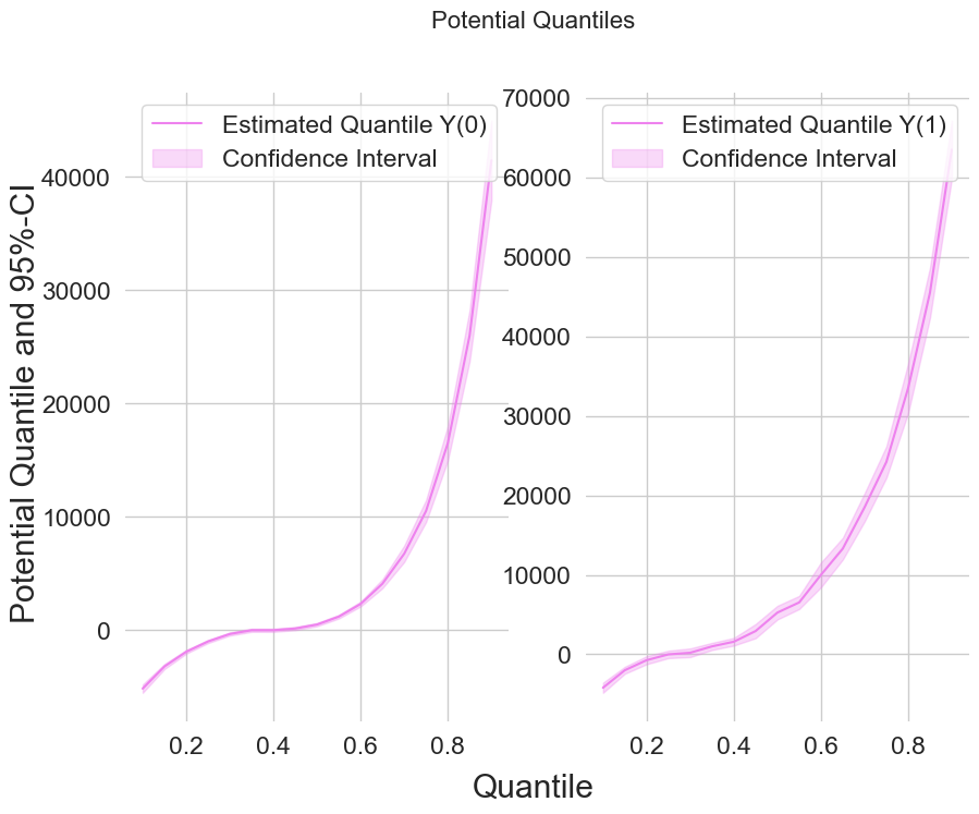
Finally, let us take a look at the estimated potential quantiles
[10]:
data_pq = {"Quantile": tau_vec,
           "DML Y(0)": PQ_0, "DML Y(1)": PQ_1,
           "DML Y(0) lower": ci_PQ_0[:, 0], "DML Y(0) upper": ci_PQ_0[:, 1],
           "DML Y(1) lower": ci_PQ_1[:, 0], "DML Y(1) upper": ci_PQ_1[:, 1]}
df_pq = pd.DataFrame(data_pq)
print(df_pq)
    Quantile      DML Y(0)      DML Y(1)  DML Y(0) lower  DML Y(0) upper  \
0       0.10 -5.320000e+03 -3.978000e+03    -5708.039154    -4931.960846
1       0.15 -3.200000e+03 -2.000000e+03    -3422.338855    -2977.661145
2       0.20 -2.000000e+03 -7.270000e+02    -2167.843296    -1832.156704
3       0.25 -1.000000e+03 -1.077527e-12    -1144.513658     -855.486342
4       0.30 -3.480000e+02  2.800000e+02     -485.671633     -210.328367
5       0.35 -1.063428e-12  1.000000e+03     -140.524215      140.524215
6       0.40  1.512657e-12  1.425000e+03     -141.848578      141.848578
7       0.45  1.000000e+02  3.648000e+03      -43.070797      243.070797
8       0.50  5.000000e+02  4.450000e+03      354.370165      645.629835
9       0.55  1.200000e+03  6.450000e+03     1040.412406     1359.587594
10      0.60  2.398000e+03  9.500000e+03     2175.942629     2620.057371
11      0.65  4.100000e+03  1.370000e+04     3712.348338     4487.651662
12      0.70  6.499000e+03  1.790000e+04     5804.239845     7193.760155
13      0.75  1.074700e+04  2.330000e+04     9773.014721    11720.985279
14      0.80  1.600000e+04  3.320000e+04    14530.490898    17469.509102
15      0.85  2.564800e+04  4.496300e+04    23368.042583    27927.957417
16      0.90  4.190000e+04  6.349900e+04    38348.193833    45451.806167

    DML Y(1) lower  DML Y(1) upper
0     -4584.205245    -3371.794755
1     -2445.618722    -1554.381278
2     -1275.916921     -178.083079
3      -412.409390      412.409390
4      -179.647750      739.647750
5       413.167035     1586.832965
6       843.522605     2006.477395
7      2760.562866     4535.437134
8      3598.463208     5301.536792
9      5494.106116     7405.893884
10     8208.841712    10791.158288
11    11850.483855    15549.516145
12    16249.111783    19550.888217
13    20956.028868    25643.971132
14    30186.784841    36213.215159
15    42143.373235    47782.626765
16    59798.135596    67199.864404
[11]:
from matplotlib import pyplot as plt
plt.rcParams['figure.figsize'] = 10., 7.5
fig, (ax1, ax2) = plt.subplots(1 ,2)
ax1.grid(visible=True); ax2.grid(visible=True)

ax1.plot(df_pq['Quantile'],df_pq['DML Y(0)'], color='violet', label='Estimated Quantile Y(0)')
ax1.fill_between(df_pq['Quantile'], df_pq['DML Y(0) lower'], df_pq['DML Y(0) upper'], color='violet', alpha=.3, label='Confidence Interval')
ax1.legend()

ax2.plot(df_pq['Quantile'],df_pq['DML Y(1)'], color='violet', label='Estimated Quantile Y(1)')
ax2.fill_between(df_pq['Quantile'], df_pq['DML Y(1) lower'], df_pq['DML Y(1) upper'], color='violet', alpha=.3, label='Confidence Interval')
ax2.legend()


fig.suptitle('Potential Quantiles', fontsize=16)
fig.supxlabel('Quantile')
_ = fig.supylabel('Potential Quantile and 95%-CI')
As we are interested in the QTE, we can use the DoubleMLQTE object, which internally fits two DoubleMLPQ objects for the treatment and control group. The main advantage is to apply this to a list of quantiles and construct uniformly valid confidence intervals for the range of treatment effects.
[12]:
n_cores = multiprocessing.cpu_count()
cores_used = np.min([5, n_cores - 1])
print(f"Number of Cores used: {cores_used}")

np.random.seed(42)
dml_QTE = dml.DoubleMLQTE(data_dml_base,
                           ml_g=clone(class_learner),
                           ml_m=clone(class_learner),
                           quantiles=tau_vec,
                           score='PQ',
                           n_folds=n_folds,
                           normalize_ipw=True,
                           trimming_rule="truncate",
                           trimming_threshold=1e-2)
dml_QTE.fit(n_jobs_models=cores_used)
print(dml_QTE)
Number of Cores used: 5
================== DoubleMLQTE Object ==================

------------------ Fit summary       ------------------
         coef      std err          t         P>|t|         2.5 %  \
0.10   1210.0   486.438569   2.487467  1.286563e-02    256.597923
0.15   1230.0   263.748513   4.663533  3.108257e-06    713.062414
0.20   1211.0   252.052811   4.804549  1.551010e-06    716.985569
0.25   1000.0   244.841847   4.084269  4.421576e-05    520.118799
0.30    622.0   255.252133   2.436806  1.481761e-02    121.715013
0.35   1031.0   274.813682   3.751633  1.756867e-04    492.375081
0.40   2006.0   320.163566   6.265547  3.715179e-10   1378.490941
0.45   3329.0   427.336461   7.790115  6.661338e-15   2491.435927
0.50   4601.0   448.109454  10.267581  0.000000e+00   3722.721609
0.55   6000.0   590.561309  10.159826  0.000000e+00   4842.521104
0.60   7040.0   605.739720  11.622153  0.000000e+00   5852.771965
0.65   9243.0   809.469379  11.418591  0.000000e+00   7656.469170
0.70  10928.0   859.705581  12.711328  0.000000e+00   9243.008023
0.75  12410.0  1018.114834  12.189195  0.000000e+00  10414.531594
0.80  16590.0  1589.396531  10.437924  0.000000e+00  13474.840041
0.85  19382.0  1622.701413  11.944280  0.000000e+00  16201.563673
0.90  21550.0  2279.055439   9.455672  0.000000e+00  17083.133421

            97.5 %
0.10   2163.402077
0.15   1746.937586
0.20   1705.014431
0.25   1479.881201
0.30   1122.284987
0.35   1569.624919
0.40   2633.509059
0.45   4166.564073
0.50   5479.278391
0.55   7157.478896
0.60   8227.228035
0.65  10829.530830
0.70  12612.991977
0.75  14405.468406
0.80  19705.159959
0.85  22562.436327
0.90  26016.866579
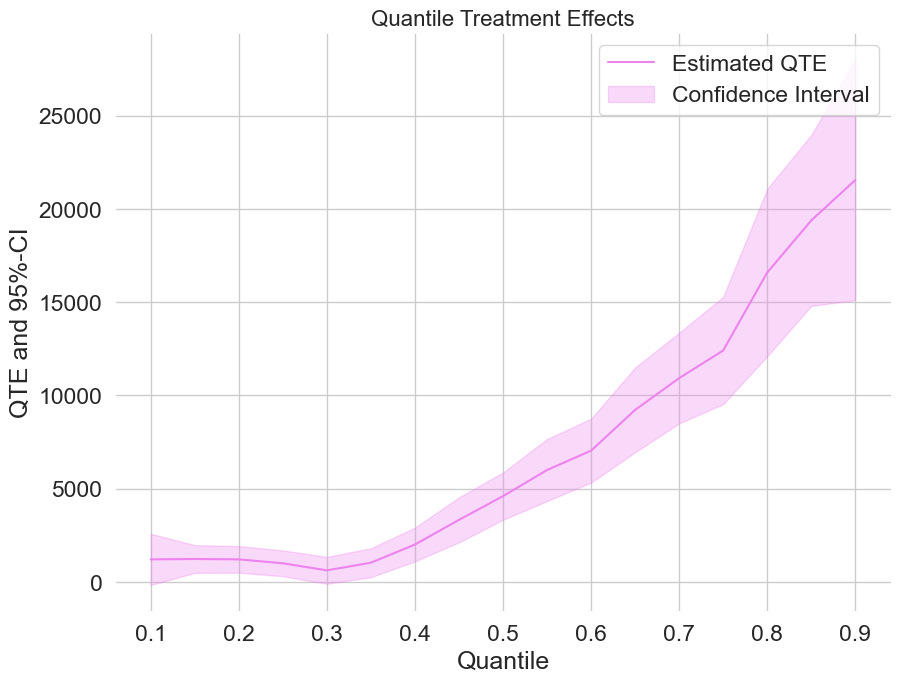
For uniformly valid confidence intervals, we still need to apply a bootstrap first. Let’s take a quick look at the QTEs combinded with a confidence interval.
[13]:
dml_QTE.bootstrap(n_rep_boot=2000)
ci_QTE = dml_QTE.confint(level=0.95, joint=True)

data_qte = {"Quantile": tau_vec, "DML QTE": dml_QTE.coef,
            "DML QTE lower": ci_QTE["2.5 %"], "DML QTE upper": ci_QTE["97.5 %"]}
df_qte = pd.DataFrame(data_qte)
print(df_qte)
      Quantile  DML QTE  DML QTE lower  DML QTE upper
0.10      0.10   1210.0    -164.794119    2584.794119
0.15      0.15   1230.0     484.582331    1975.417669
0.20      0.20   1211.0     498.637240    1923.362760
0.25      0.25   1000.0     308.017185    1691.982815
0.30      0.30    622.0     -99.404824    1343.404824
0.35      0.35   1031.0     254.309464    1807.690536
0.40      0.40   2006.0    1101.139622    2910.860378
0.45      0.45   3329.0    2121.242864    4536.757136
0.50      0.50   4601.0    3334.533316    5867.466684
0.55      0.55   6000.0    4330.929607    7669.070393
0.60      0.60   7040.0    5328.031712    8751.968288
0.65      0.65   9243.0    6955.241973   11530.758027
0.70      0.70  10928.0    8498.262204   13357.737796
0.75      0.75  12410.0    9532.558996   15287.441004
0.80      0.80  16590.0   12097.977489   21082.022511
0.85      0.85  19382.0   14795.849766   23968.150234
0.90      0.90  21550.0   15108.833096   27991.166904
[14]:
plt.rcParams['figure.figsize'] = 10., 7.5
fig, ax = plt.subplots()
ax.grid(visible=True)


ax.plot(df_qte['Quantile'],df_qte['DML QTE'], color='violet', label='Estimated QTE')
ax.fill_between(df_qte['Quantile'], df_qte['DML QTE lower'], df_qte['DML QTE upper'], color='violet', alpha=.3, label='Confidence Interval')


plt.legend()
plt.title('Quantile Treatment Effects', fontsize=16)
plt.xlabel('Quantile')
_ = plt.ylabel('QTE and 95%-CI')
Estimating the treatment effect on the Conditional Value a Risk (CVaR)#
Similar to the evaluation of the estimation of quantile treatment effects (QTEs), we can estimate the conditional value at risk (CVaR) for given quantiles. Here, we will only focus on treatment effect estimation, but the DoubleML package also allows for estimation of potential CVaRs.
The estimation of treatment effects can be easily done by adjusting the score in the DoubleMLQTE object to score="CVaR", as the estimation is based on the same nuisance elements as QTEs.
[15]:
np.random.seed(42)
dml_CVAR = dml.DoubleMLQTE(data_dml_base,
                           ml_g=clone(reg_learner),
                           ml_m=clone(class_learner),
                           quantiles=tau_vec,
                           score="CVaR",
                           n_folds=n_folds,
                           normalize_ipw=True,
                           trimming_rule="truncate",
                           trimming_threshold=1e-2)
dml_CVAR.fit(n_jobs_models=cores_used)
print(dml_CVAR)
================== DoubleMLQTE Object ==================

------------------ Fit summary       ------------------
              coef       std err          t         P>|t|         2.5 %  \
0.10   9045.771876   1297.433473   6.972051  3.123501e-12   6502.848997
0.15  10126.150435   1371.682315   7.382285  1.556533e-13   7437.702500
0.20  14588.483642   1485.887212   9.818029  0.000000e+00  11676.198221
0.25  16910.113005   1582.022950  10.688918  0.000000e+00  13809.405000
0.30  14744.693345   1676.606733   8.794366  0.000000e+00  11458.604532
0.35  16241.220211   1812.325046   8.961538  0.000000e+00  12689.128393
0.40  18666.064164   1970.604110   9.472255  0.000000e+00  14803.751081
0.45  12861.546438   2086.920695   6.162930  7.141101e-10   8771.257037
0.50  13642.272643   2295.693359   5.942550  2.806220e-09   9142.796340
0.55  14772.076119   2543.121297   5.808640  6.298235e-09   9787.649969
0.60  15556.470365   2849.994864   5.458420  4.803889e-08   9970.583076
0.65  16618.635757   3235.158198   5.136885  2.793297e-07  10277.842205
0.70  17576.744211   3745.384883   4.692907  2.693495e-06  10235.924732
0.75  18773.183814   4438.392472   4.229726  2.339762e-05  10074.094420
0.80  19798.478399   5475.067639   3.616116  2.990567e-04   9067.543014
0.85  19824.886611   7155.563760   2.770556  5.596076e-03   5800.239352
0.90  20055.810916  10406.538282   1.927232  5.395076e-02   -340.629319

            97.5 %
0.10  11588.694755
0.15  12814.598371
0.20  17500.769063
0.25  20010.821009
0.30  18030.782159
0.35  19793.312030
0.40  22528.377246
0.45  16951.835839
0.50  18141.748945
0.55  19756.502268
0.60  21142.357654
0.65  22959.429309
0.70  24917.563690
0.75  27472.273208
0.80  30529.413784
0.85  33849.533871
0.90  40452.251152
Estimation of the corresponding (uniformly) valid confidence intervals can be done analogously to the quantile treatment effects.
[16]:
dml_CVAR.bootstrap(n_rep_boot=2000)
ci_CVAR = dml_CVAR.confint(level=0.95, joint=True)

data_cvar = {"Quantile": tau_vec, "DML CVAR": dml_CVAR.coef,
            "DML CVAR lower": ci_CVAR["2.5 %"], "DML CVAR upper": ci_CVAR["97.5 %"]}
df_cvar = pd.DataFrame(data_cvar)
print(df_cvar)
      Quantile      DML CVAR  DML CVAR lower  DML CVAR upper
0.10      0.10   9045.771876     6241.250083    11850.293669
0.15      0.15  10126.150435     7161.132941    13091.167930
0.20      0.20  14588.483642    11376.601757    17800.365527
0.25      0.25  16910.113005    13490.424879    20329.801130
0.30      0.30  14744.693345    11120.553672    18368.833018
0.35      0.35  16241.220211    12323.712921    20158.727501
0.40      0.40  18666.064164    14406.422119    22925.706208
0.45      0.45  12861.546438     8350.475395    17372.617481
0.50      0.50  13642.272643     8679.920283    18604.625002
0.55      0.55  14772.076119     9274.885513    20269.266724
0.60      0.60  15556.470365     9395.944317    21716.996413
0.65      0.65  16618.635757     9625.543734    23611.727780
0.70      0.70  17576.744211     9480.750275    25672.738147
0.75      0.75  18773.183814     9179.190231    28367.177397
0.80      0.80  19798.478399     7963.616086    31633.340712
0.85      0.85  19824.886611     4357.477354    35292.295868
0.90      0.90  20055.810916    -2438.878802    42550.500635
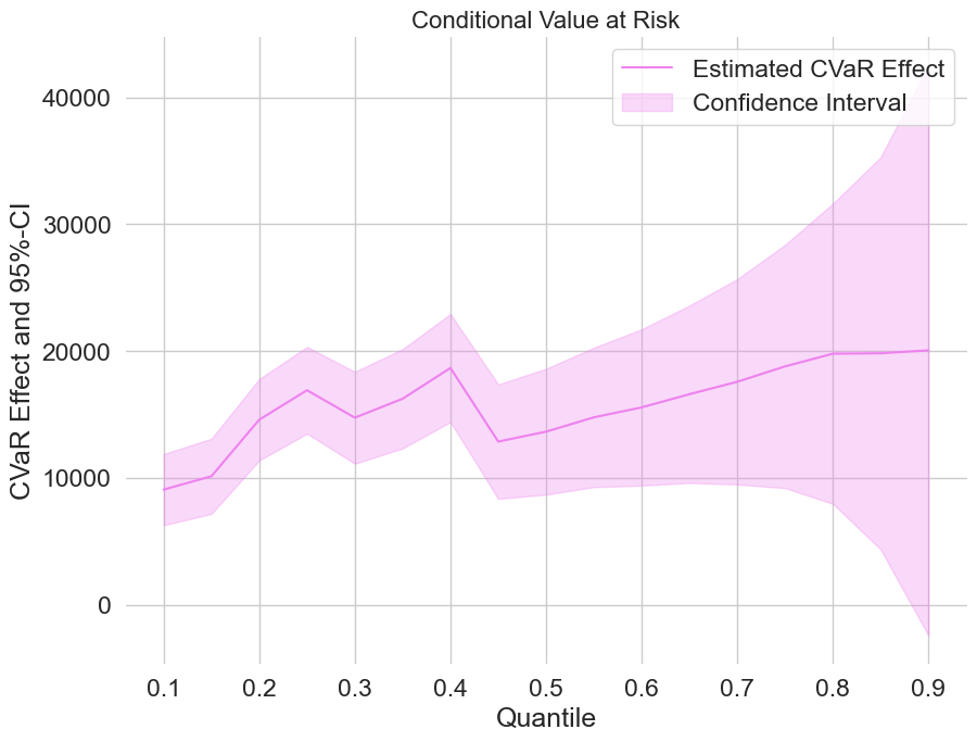
Finally, let us take a look at the estimated treatment effects on the CVaR.
[17]:
plt.rcParams['figure.figsize'] = 10., 7.5
fig, ax = plt.subplots()
ax.grid(visible=True)

ax.plot(df_cvar['Quantile'],df_cvar['DML CVAR'], color='violet', label='Estimated CVaR Effect')
ax.fill_between(df_cvar['Quantile'], df_cvar['DML CVAR lower'], df_cvar['DML CVAR upper'], color='violet', alpha=.3, label='Confidence Interval')

plt.legend()
plt.title('Conditional Value at Risk', fontsize=16)
plt.xlabel('Quantile')
_ = plt.ylabel('CVaR Effect and 95%-CI')
Estimating local quantile treatment effects (LQTEs)#
If we have an IIVM model with a given instrumental variable, we are still able to identify the local quantile treatment effect (LQTE), the quantile treatment effect on compliers. For the 401(k) pension data we can use e401 as an instrument for participation p401. To fit an DoubleML model with an instrument, we have to change the data backend and specify the instrument.
[18]:
# Initialize DoubleMLData with an instrument

# Basic model
data_dml_base_iv = dml.DoubleMLData(data,
                                    y_col='net_tfa',
                                    d_cols='p401',
                                    z_cols='e401',
                                    x_cols=features_base)

print(data_dml_base_iv)
================== DoubleMLData Object ==================

------------------ Data summary      ------------------
Outcome variable: net_tfa
Treatment variable(s): ['p401']
Covariates: ['age', 'inc', 'educ', 'fsize', 'marr', 'twoearn', 'db', 'pira', 'hown']
Instrument variable(s): ['e401']
No. Observations: 9915

------------------ DataFrame info    ------------------
<class 'pandas.core.frame.DataFrame'>
RangeIndex: 9915 entries, 0 to 9914
Columns: 14 entries, nifa to hown
dtypes: float32(4), int8(10)
memory usage: 251.9 KB
The estimation of local treatment effects can be easily done by adjusting the score in the DoubleMLQTE object to score="LPQ".
[19]:
np.random.seed(42)
dml_LQTE = dml.DoubleMLQTE(data_dml_base_iv,
                           ml_g=clone(class_learner),
                           ml_m=clone(class_learner),
                           quantiles=tau_vec,
                           score="LPQ",
                           n_folds=n_folds,
                           normalize_ipw=True,
                           trimming_rule="truncate",
                           trimming_threshold=1e-2)
dml_LQTE.fit(n_jobs_models=cores_used)
print(dml_LQTE)
================== DoubleMLQTE Object ==================

------------------ Fit summary       ------------------
         coef      std err          t         P>|t|         2.5 %  \
0.10   2610.0   487.820993   5.350323  8.779727e-08   1653.888423
0.15   1773.0   357.148835   4.964317  6.894329e-07   1073.001145
0.20   1398.0   386.526532   3.616828  2.982353e-04    640.421919
0.25   1435.0   384.956574   3.727693  1.932404e-04    680.498979
0.30   1400.0   436.977295   3.203828  1.356136e-03    543.540240
0.35   2500.0   486.877153   5.134765  2.824961e-07   1545.738315
0.40   3985.0   596.725087   6.678117  2.420308e-11   2815.440320
0.45   5175.0   739.887778   6.994304  2.665868e-12   3724.846602
0.50   7239.0   775.751013   9.331602  0.000000e+00   5718.555954
0.55   9500.0  1109.046788   8.565915  0.000000e+00   7326.308239
0.60  11750.0  1295.711518   9.068377  0.000000e+00   9210.452091
0.65  14625.0  1443.080854  10.134567  0.000000e+00  11796.613498
0.70  16984.0  1576.564577  10.772791  0.000000e+00  13893.990210
0.75  19758.0  2865.426736   6.895308  5.374812e-12  14141.866798
0.80  23856.0  2281.099670  10.458114  0.000000e+00  19385.126802
0.85  27066.0  2920.063312   9.268977  0.000000e+00  21342.781076
0.90  30645.0  4634.200110   6.612792  3.771383e-11  21562.134687

            97.5 %
0.10   3566.111577
0.15   2472.998855
0.20   2155.578081
0.25   2189.501021
0.30   2256.459760
0.35   3454.261685
0.40   5154.559680
0.45   6625.153398
0.50   8759.444046
0.55  11673.691761
0.60  14289.547909
0.65  17453.386502
0.70  20074.009790
0.75  25374.133202
0.80  28326.873198
0.85  32789.218924
0.90  39727.865313
Estimation of the corresponding (uniformly) valid confidence intervals can be done analogously to the quantile treatment effects.
[20]:
dml_LQTE.bootstrap(n_rep_boot=2000)
ci_LQTE = dml_LQTE.confint(level=0.95, joint=True)

data_lqte = {"Quantile": tau_vec, "DML LQTE": dml_LQTE.coef,
            "DML LQTE lower": ci_LQTE["2.5 %"], "DML LQTE upper": ci_LQTE["97.5 %"]}
df_lqte = pd.DataFrame(data_lqte)
print(df_lqte)
      Quantile  DML LQTE  DML LQTE lower  DML LQTE upper
0.10      0.10    2610.0     1258.618753     3961.381247
0.15      0.15    1773.0      783.611995     2762.388005
0.20      0.20    1398.0      327.228725     2468.771275
0.25      0.25    1435.0      368.577884     2501.422116
0.30      0.30    1400.0      189.468001     2610.531999
0.35      0.35    2500.0     1151.233415     3848.766585
0.40      0.40    3985.0     2331.928269     5638.071731
0.45      0.45    5175.0     3125.333250     7224.666750
0.50      0.50    7239.0     5089.983482     9388.016518
0.55      0.55    9500.0     6427.674181    12572.325819
0.60      0.60   11750.0     8160.568071    15339.431929
0.65      0.65   14625.0    10627.319634    18622.680366
0.70      0.70   16984.0    12616.537681    21351.462319
0.75      0.75   19758.0    11820.080121    27695.919879
0.80      0.80   23856.0    17536.806356    30175.193644
0.85      0.85   27066.0    18976.723689    35155.276311
0.90      0.90   30645.0    17807.153293    43482.846707
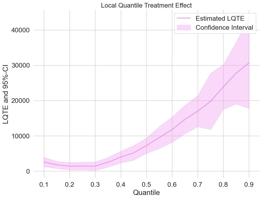
Finally, let us take a look at the estimated local quantile treatment effects.
[21]:
plt.rcParams['figure.figsize'] = 10., 7.5
fig, ax = plt.subplots()
ax.grid(visible=True)

ax.plot(df_lqte['Quantile'],df_lqte['DML LQTE'], color='violet', label='Estimated LQTE')
ax.fill_between(df_lqte['Quantile'], df_lqte['DML LQTE lower'], df_lqte['DML LQTE upper'], color='violet', alpha=.3, label='Confidence Interval')

plt.legend()
plt.title('Local Quantile Treatment Effect', fontsize=16)
plt.xlabel('Quantile')
_ = plt.ylabel('LQTE and 95%-CI')