Note
-
Download Jupyter notebook:
https://docs.doubleml.org/stable/examples/py_double_ml_irm_vs_apo.ipynb.
Python: IRM and APO Model Comparison#
In this simple example, we illustrate how the (binary) DoubleMLIRM class relates to the DoubleMLAPOS class.
More specifically, we focus on the causal_contrast() method of DoubleMLAPOS in a binary setting to highlight, when both methods coincide.
[1]:
import numpy as np
import pandas as pd
import doubleml as dml

from sklearn.linear_model import LinearRegression, LogisticRegression
from sklearn.preprocessing import PolynomialFeatures

from matplotlib import pyplot as plt

from doubleml.irm.datasets import make_irm_data
Data#
We rely on the make_irm_data go generate data with a binary treatment.
[2]:
n_obs = 2000

np.random.seed(42)
df = make_irm_data(
    n_obs=n_obs,
    dim_x=10,
    theta=5.0,
    return_type='DataFrame'
)

df.head()
[2]:
| X1 | X2 | X3 | X4 | X5 | X6 | X7 | X8 | X9 | X10 | y | d | |
|---|---|---|---|---|---|---|---|---|---|---|---|---|
| 0 | 0.541060 | 0.195963 | 0.835750 | 1.180271 | 0.655959 | 1.044239 | -1.214769 | -2.160836 | -2.196655 | -2.037529 | 4.704558 | 1.0 |
| 1 | 1.340235 | 2.319420 | 2.193375 | 1.139508 | 1.458814 | 0.493195 | 1.313870 | 0.127337 | 0.418400 | 1.070433 | 6.113952 | 1.0 |
| 2 | -0.563563 | -1.480199 | 0.943548 | -0.400113 | 0.757559 | 0.131483 | -0.574160 | 0.067212 | -0.427654 | -1.342117 | -0.226479 | 0.0 |
| 3 | -0.044176 | -2.122421 | -1.526582 | -1.892828 | -1.777867 | -1.425325 | 0.020272 | 0.487524 | -0.579197 | -0.752909 | 0.367366 | 0.0 |
| 4 | -1.896263 | -1.198493 | -1.285483 | -1.361623 | -2.921778 | -2.026966 | -1.107156 | -0.498122 | 0.568287 | 1.004542 | 0.913585 | 0.0 |
First, define the DoubleMLData object.
[3]:
dml_data = dml.DoubleMLData(
    df,
    y_col='y',
    d_cols='d'
)
Learners and Hyperparameters#
To simplify the comparison and keep the variation in learners as small as possible, we will use linear models.
[4]:
n_folds = 5
n_rep = 1

dml_kwargs = {
    "obj_dml_data": dml_data,
    "ml_g": LinearRegression(),
    "ml_m": LogisticRegression(random_state=42),
    "n_folds": n_folds,
    "n_rep": n_rep,
    "normalize_ipw": False,
    "trimming_threshold": 1e-2,
    "draw_sample_splitting": False,
}
Remark: All results rely on the exact same predictions for the machine learning algorithms. If the more than two treatment levels exists the DoubleMLAPOS model fit multiple binary models such that the combined model might differ.
Further, to remove all uncertainty from sample splitting, we will rely on externally provided sample splits.
[5]:
from doubleml.utils import DoubleMLResampling

rskf = DoubleMLResampling(
    n_folds=n_folds,
    n_rep=n_rep,
    n_obs=n_obs,
    stratify=df['d'],
)
all_smpls = rskf.split_samples()
Average Treatment Effect#
Comparing the effect estimates for the DoubleMLIRM and causal_contrasts of the DoubleMLAPOS model, we can numerically equivalent results for the ATE.
[6]:
dml_irm = dml.DoubleMLIRM(**dml_kwargs)
dml_irm.set_sample_splitting(all_smpls)
print("Training IRM Model")
dml_irm.fit()

print(dml_irm.summary)
Training IRM Model
       coef   std err          t  P>|t|     2.5 %    97.5 %
d  5.001907  0.066295  75.449677    0.0  4.871972  5.131842
[7]:
dml_apos = dml.DoubleMLAPOS(treatment_levels=[0,1], **dml_kwargs)
dml_apos.set_sample_splitting(all_smpls)
print("Training APOS Model")
dml_apos.fit()
print(dml_apos.summary)

print("Evaluate Causal Contrast")
causal_contrast = dml_apos.causal_contrast(reference_levels=[0])
print(causal_contrast.summary)
Training APOS Model
       coef   std err           t    P>|t|     2.5 %    97.5 %
0  0.038103  0.045984    0.828618  0.40732 -0.052023  0.128229
1  5.040010  0.047873  105.278454  0.00000  4.946180  5.133839
Evaluate Causal Contrast
            coef   std err          t  P>|t|     2.5 %    97.5 %
1 vs 0  5.001907  0.066295  75.449677    0.0  4.871972  5.131842
For a direct comparison, see
[8]:
print("IRM Model")
print(dml_irm.summary)
print("Causal Contrast")
print(causal_contrast.summary)
IRM Model
       coef   std err          t  P>|t|     2.5 %    97.5 %
d  5.001907  0.066295  75.449677    0.0  4.871972  5.131842
Causal Contrast
            coef   std err          t  P>|t|     2.5 %    97.5 %
1 vs 0  5.001907  0.066295  75.449677    0.0  4.871972  5.131842
Average Treatment Effect on the Treated#
For the average treatment effect on the treated we can adjust the score in DoubleMLIRM model to score="ATTE".
[9]:
dml_irm_atte = dml.DoubleMLIRM(score="ATTE", **dml_kwargs)
dml_irm_atte.set_sample_splitting(all_smpls)
print("Training IRM Model")
dml_irm_atte.fit()

print(dml_irm_atte.summary)
Training IRM Model
       coef  std err          t  P>|t|     2.5 %    97.5 %
d  5.540549  0.08364  66.242427    0.0  5.376617  5.704482
In order to consider weighted effects in the DoubleMLAPOS model, we have to specify the correct weight, see User Guide.
As these weights include the propensity score, we will use the predicted propensity score from the previous DoubleMLIRM model.
[10]:
p_hat = df["d"].mean()
m_hat = dml_irm_atte.predictions["ml_m"][:, :, 0]

weights_dict = {
    "weights": df["d"] / p_hat,
    "weights_bar": m_hat / p_hat,
}

dml_apos_atte = dml.DoubleMLAPOS(treatment_levels=[0,1], weights=weights_dict, **dml_kwargs)
dml_apos_atte.set_sample_splitting(all_smpls)
print("Training APOS Model")
dml_apos_atte.fit()
print(dml_apos_atte.summary)

print("Evaluate Causal Contrast")
causal_contrast_atte = dml_apos_atte.causal_contrast(reference_levels=[0])
print(causal_contrast_atte.summary)
Training APOS Model
       coef   std err           t     P>|t|     2.5 %    97.5 %
0  0.044929  0.073384    0.612246  0.540375 -0.098901  0.188760
1  5.585479  0.039895  140.003045  0.000000  5.507285  5.663672
Evaluate Causal Contrast
            coef  std err          t  P>|t|     2.5 %    97.5 %
1 vs 0  5.540549  0.08364  66.242427    0.0  5.376617  5.704482
The same results can be achieved by specifying the weights for DoubleMLIRM class with score='ATE'.
[11]:
dml_irm_weighted_atte = dml.DoubleMLIRM(score="ATE", weights=weights_dict, **dml_kwargs)
dml_irm_weighted_atte.set_sample_splitting(all_smpls)
print("Training IRM Model")
dml_irm_weighted_atte.fit()

print(dml_irm_weighted_atte.summary)
Training IRM Model
       coef  std err          t  P>|t|     2.5 %    97.5 %
d  5.540549  0.08364  66.242427    0.0  5.376617  5.704482
In summary, see
[12]:
print("IRM Model ATTE Score")
print(dml_irm_atte.summary.round(4))
print("IRM Model (Weighted)")
print(dml_irm_weighted_atte.summary.round(4))
print("Causal Contrast (Weighted)")
print(causal_contrast_atte.summary.round(4))
IRM Model ATTE Score
     coef  std err        t  P>|t|   2.5 %  97.5 %
d  5.5405   0.0836  66.2424    0.0  5.3766  5.7045
IRM Model (Weighted)
     coef  std err        t  P>|t|   2.5 %  97.5 %
d  5.5405   0.0836  66.2424    0.0  5.3766  5.7045
Causal Contrast (Weighted)
          coef  std err        t  P>|t|   2.5 %  97.5 %
1 vs 0  5.5405   0.0836  66.2424    0.0  5.3766  5.7045
Sensitivity Analysis#
The sensitvity analysis gives identical results.
[13]:
dml_irm.sensitivity_analysis()
print(dml_irm.sensitivity_summary)
================== Sensitivity Analysis ==================

------------------ Scenario          ------------------
Significance Level: level=0.95
Sensitivity parameters: cf_y=0.03; cf_d=0.03, rho=1.0

------------------ Bounds with CI    ------------------
   CI lower  theta lower     theta  theta upper  CI upper
d  4.773339     4.890665  5.001907     5.113149  5.217684

------------------ Robustness Values ------------------
   H_0     RV (%)    RVa (%)
d  0.0  72.206256  66.239019
[14]:
causal_contrast.sensitivity_analysis()
print(causal_contrast.sensitivity_summary)
================== Sensitivity Analysis ==================

------------------ Scenario          ------------------
Significance Level: level=0.95
Sensitivity parameters: cf_y=0.03; cf_d=0.03, rho=1.0

------------------ Bounds with CI    ------------------
        CI lower  theta lower     theta  theta upper  CI upper
1 vs 0  4.773339     4.890665  5.001907     5.113149  5.217684

------------------ Robustness Values ------------------
        H_0     RV (%)    RVa (%)
1 vs 0  0.0  72.206256  66.239019
Effect Heterogeneity#
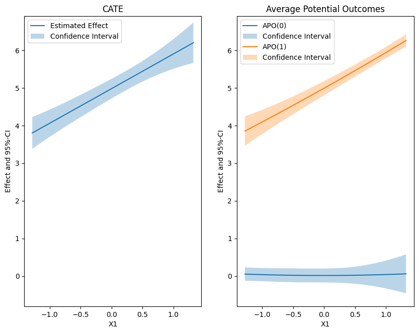
For conditional treatment effects the exact same methods do not exist. Nevertheless, we will compare the capo() variant of the DoubleMLAPO class to the corresponding cate() method of the DoubleMLIRM class.
For a simple case we will just use a polynomial basis of the first feature X1. To plot the data we will evaluate the methods on the corresponding grid of basis values.
[15]:
X = df[["X1"]]
poly = PolynomialFeatures(degree=2, include_bias=True)

basis_matrix = poly.fit_transform(X)
basis_df = pd.DataFrame(basis_matrix, columns=poly.get_feature_names_out(["X1"]))

grid = pd.DataFrame({"X1": np.linspace(np.quantile(df["X1"], 0.1), np.quantile(df["X1"], 0.9), 100)})
grid_basis = pd.DataFrame( poly.transform(grid), columns=poly.get_feature_names_out(["X1"]))
Apply the cate() method to the basis and evaluate on the transformed grid values.
[16]:
cate = dml_irm.cate(basis_df)
print(cate)
np.random.seed(42)
df_cate = cate.confint(grid_basis, level=0.95, joint=True, n_rep_boot=2000)
================== DoubleMLBLP Object ==================

------------------ Fit summary ------------------
          coef   std err          t         P>|t|    [0.025    0.975]
1     4.979966  0.065976  75.481713  0.000000e+00  4.850656  5.109277
X1    0.921198  0.072516  12.703325  5.666959e-37  0.779068  1.063327
X1^2  0.001698  0.042804   0.039661  9.683637e-01 -0.082197  0.085592
The corresponding apo() method can be used for the treatment levels \(0\) and \(1\).
[17]:
capo0 = dml_apos.modellist[0].capo(basis_df)
print(capo0)
np.random.seed(42)
df_capo0 = capo0.confint(grid_basis, level=0.95, joint=True, n_rep_boot=2000)

capo1 = dml_apos.modellist[1].capo(basis_df)
print(capo1)
np.random.seed(42)
df_capo1 = capo1.confint(grid_basis, level=0.95, joint=True, n_rep_boot=2000)
================== DoubleMLBLP Object ==================

------------------ Fit summary ------------------
          coef   std err         t     P>|t|    [0.025    0.975]
1     0.013450  0.046451  0.289555  0.772157 -0.077592  0.104492
X1    0.001471  0.056915  0.025841  0.979384 -0.110081  0.113022
X1^2  0.024266  0.037114  0.653829  0.513222 -0.048476  0.097009
================== DoubleMLBLP Object ==================

------------------ Fit summary ------------------
          coef   std err           t         P>|t|    [0.025    0.975]
1     4.993416  0.047239  105.704896  0.000000e+00  4.900829  5.086004
X1    0.922668  0.045172   20.425636  9.896182e-93  0.834133  1.011204
X1^2  0.025964  0.022258    1.166517  2.434054e-01 -0.017660  0.069589
In this example the average potential outcome of the control group is zero (as can be seen in the outcome definition, see documentation). Let us visualize the effects
[18]:
df_cate['x'] = grid_basis['X1']

plt.rcParams['figure.figsize'] = 10., 7.5
fig, (ax1, ax2) = plt.subplots(1, 2)

# Plot CATE
ax1.plot(df_cate['x'], df_cate['effect'], label='Estimated Effect')
ax1.fill_between(df_cate['x'], df_cate['2.5 %'], df_cate['97.5 %'], alpha=.3, label='Confidence Interval')
ax1.legend()
ax1.set_title('CATE')
ax1.set_xlabel('X1')
ax1.set_ylabel('Effect and 95%-CI')

# Plot Average Potential Outcomes
ax2.plot(df_cate['x'], df_capo0['effect'], label='APO(0)')
ax2.fill_between(df_cate['x'], df_capo0['2.5 %'], df_capo0['97.5 %'], alpha=.3, label='Confidence Interval')
ax2.plot(df_cate['x'], df_capo1['effect'], label='APO(1)')
ax2.fill_between(df_cate['x'], df_capo1['2.5 %'], df_capo1['97.5 %'], alpha=.3, label='Confidence Interval')
ax2.legend()
ax2.set_title('Average Potential Outcomes')
ax2.set_xlabel('X1')
ax2.set_ylabel('Effect and 95%-CI')

# Ensure the same scale on y-axis
ax1.set_ylim(min(ax1.get_ylim()[0], ax2.get_ylim()[0]), max(ax1.get_ylim()[1], ax2.get_ylim()[1]))
ax2.set_ylim(min(ax1.get_ylim()[0], ax2.get_ylim()[0]), max(ax1.get_ylim()[1], ax2.get_ylim()[1]))

plt.show()
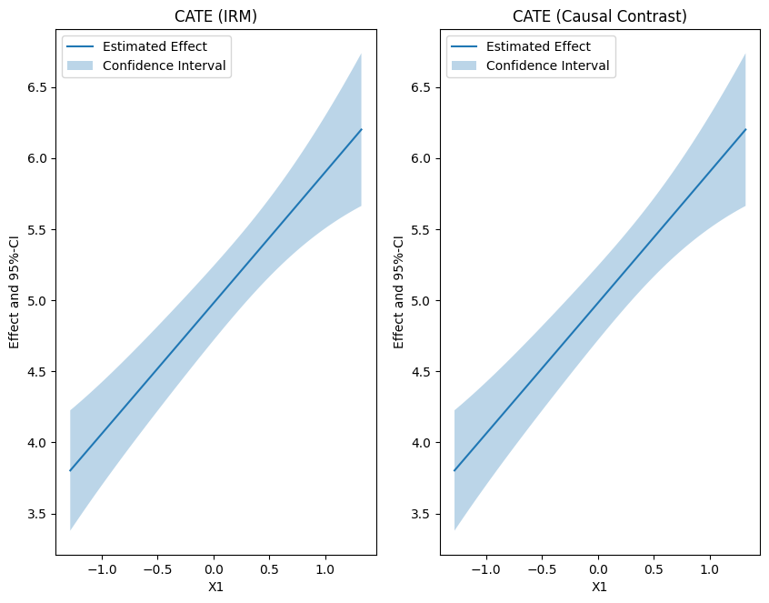
The causal_contrast() method does not currently not have a cate() method implemented. But the cate can be manually constructed via the the correct score function.
[19]:
orth_signal = -1.0 * (causal_contrast.scaled_psi.reshape(-1) - causal_contrast.thetas)

causal_contrast_cate = dml.utils.DoubleMLBLP(orth_signal, basis_df)
causal_contrast_cate.fit()
print(causal_contrast_cate.summary)
np.random.seed(42)
df_causal_contrast_cate = causal_contrast_cate.confint(grid_basis, level=0.95, joint=True, n_rep_boot=2000)

print("CATE (IRM) as comparison:")
print(cate.summary)
          coef   std err          t         P>|t|    [0.025    0.975]
1     4.979966  0.065976  75.481713  0.000000e+00  4.850656  5.109277
X1    0.921198  0.072516  12.703325  5.666959e-37  0.779068  1.063327
X1^2  0.001698  0.042804   0.039661  9.683637e-01 -0.082197  0.085592
CATE (IRM) as comparison:
          coef   std err          t         P>|t|    [0.025    0.975]
1     4.979966  0.065976  75.481713  0.000000e+00  4.850656  5.109277
X1    0.921198  0.072516  12.703325  5.666959e-37  0.779068  1.063327
X1^2  0.001698  0.042804   0.039661  9.683637e-01 -0.082197  0.085592
[20]:
plt.rcParams['figure.figsize'] = 10., 7.5
fig, (ax1, ax2) = plt.subplots(1, 2)

# Plot CATE
ax1.plot(df_cate['x'], df_cate['effect'], label='Estimated Effect')
ax1.fill_between(df_cate['x'], df_cate['2.5 %'], df_cate['97.5 %'], alpha=.3, label='Confidence Interval')
ax1.legend()
ax1.set_title('CATE (IRM)')
ax1.set_xlabel('X1')
ax1.set_ylabel('Effect and 95%-CI')

# Plot Average Potential Outcomes
ax2.plot(df_cate['x'], df_causal_contrast_cate['effect'], label='Estimated Effect')
ax2.fill_between(df_cate['x'], df_causal_contrast_cate['2.5 %'], df_causal_contrast_cate['97.5 %'], alpha=.3, label='Confidence Interval')
ax2.legend()
ax2.set_title('CATE (Causal Contrast)')
ax2.set_xlabel('X1')
ax2.set_ylabel('Effect and 95%-CI')

# Ensure the same scale on y-axis
ax1.set_ylim(min(ax1.get_ylim()[0], ax2.get_ylim()[0]), max(ax1.get_ylim()[1], ax2.get_ylim()[1]))
ax2.set_ylim(min(ax1.get_ylim()[0], ax2.get_ylim()[0]), max(ax1.get_ylim()[1], ax2.get_ylim()[1]))

plt.show()