Note

Download Jupyter notebook: https://docs.doubleml.org/stable/examples/py_double_ml_sensitivity_booking.ipynb.

Example: Sensitivity Analysis for Causal ML

This notebook complements the introductory paper “Sensitivity Analysis for Causal ML: A Use Case at Booking.com” by Bach et al. (2024) (forthcoming). It illustrates the causal analysis and sensitivity considerations in a simplified example.

import doubleml as dml
from doubleml.datasets import make_confounded_irm_data

import numpy as np
import pandas as pd
import matplotlib.pyplot as plt
import seaborn as sns

from sklearn.linear_model import LinearRegression, LogisticRegression
from sklearn.ensemble import RandomForestRegressor, RandomForestClassifier
from sklearn.isotonic import IsotonicRegression
from lightgbm import LGBMRegressor, LGBMClassifier
import plotly.graph_objects as go

Load Data

We will simulate a data set according to a data generating process (DGP), which is available and documented in the DoubleML for Python. We will parametrize the DGP in a way that it roughly mimics patterns of the data used in the original analysis.

# Use smaller number of observations in demo example to reduce computational time
n_obs = 75000

# Parameters for the data generating process
# True average treatment effect (very similar to ATT in this example)
theta = 0.07
# Coefficient of the unobserved confounder in the outcome regression.
beta_a = 0.25
# Coefficient of the unobserved confounder in the propensity score.
gamma_a = 0.123
# Variance for outcome regression error
var_eps = 1.5
# Threshold being applied on trimming propensity score on the population level
trimming_threshold = 0.05

# Number of observations
np.random.seed(42)
dgp_dict = make_confounded_irm_data(n_obs=n_obs, theta=theta, beta_a=beta_a, gamma_a=gamma_a, var_eps=var_eps, trimming_threshold=trimming_threshold)

x_cols = [f'X{i + 1}' for i in np.arange(dgp_dict['x'].shape[1])]
df = pd.DataFrame(np.column_stack((dgp_dict['x'], dgp_dict['y'], dgp_dict['d'])), columns=x_cols + ['y', 'd'])

/home/runner/work/doubleml-docs/doubleml-docs/doubleml-for-py/doubleml/datasets.py:1050: UserWarning: Propensity score is close to 0 or 1. Trimming is at 0.05 and 0.95 is applied
  warnings.warn(f'Propensity score is close to 0 or 1. '

df.head()

	X1	X2	X3	X4	X5	y	d
0	0.496714	-0.138264	0.647689	1.523030	-0.234153	1.421200	1.0
1	-0.234137	1.579213	0.767435	-0.469474	0.542560	1.315031	1.0
2	-0.463418	-0.465730	0.241962	-1.913280	-1.724918	1.493144	1.0
3	-0.562288	-1.012831	0.314247	-0.908024	-1.412304	1.399858	1.0
4	1.465649	-0.225776	0.067528	-1.424748	-0.544383	3.092229	0.0

Causal Analysis with DoubleML

1. Formulation of Causal Model & Identification Assumptions

In the use case, we focused on a nonparametric model for the treatment effect, also called Interactive Regression Model (IRM). Under the assumptions of consistency, overlap and unconfoundedness, this model can be used to identify the Average Treatment Effect (ATE) and the Average Treatment Effect on the Treated (ATT). The identification strategy was based on a DAG.

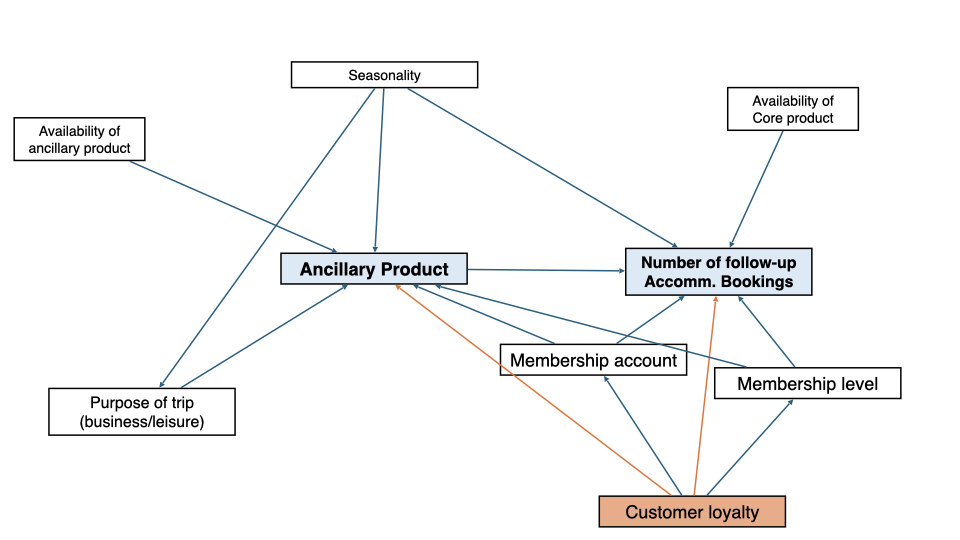
In the use case of consideration, the key causal quantity was the ATT as it quantifies by how much ancillary products increase follow-up bookings on average for customers who purchased an ancillary product.

# Set up the data backend with treatment variable d, outcome variable y, and covariates x
dml_data = dml.DoubleMLData(df, 'y', 'd', x_cols)

2. Estimation of Causal Effect

For estimation, we employed the DoubleML package in Python. The nuisance functions (including the outcome regression and the propensity score) have been used with LightGBM.

# Initialize LightGBM learners
n_estimators = 150
learning_rate = 0.05
ml_g = LGBMRegressor(n_estimators=n_estimators, learning_rate = 0.05, verbose=-1)
ml_m = LGBMClassifier(n_estimators=n_estimators, learning_rate = 0.05, verbose=-1)

# Initialize the DoubleMLIRM model, specify score "ATTE" for average treatment effect on the treated
dml_obj = dml.DoubleMLIRM(dml_data, score = "ATTE", ml_g = ml_g, ml_m = ml_m, n_folds = 5, n_rep = 2)


# fit the model
dml_obj.fit()

<doubleml.irm.irm.DoubleMLIRM at 0x7f418f2557c0>

Let’s summarize the estimation results for the ATT.

dml_obj.summary.round(3)

	coef	std err	t	P>|t|	2.5 %	97.5 %
d	0.123	0.008	15.065	0.0	0.107	0.139

The results point at a sizeable positive effect. However, we are concerned that this effect might be driven by unobserved confounders: The large positive effect might represent selection into treatment mechanisms rather than the pure causal effect of the treatment.

3. Sensitivity Analysis

To address the concerns with regard to the confounding bias, sensitivity analysis has been employed. The literature has developed various approaches, which differ in terms of their applicability to the specific estimation approach (among others). In the context of the use case, the approaches of VanderWeele and Arah (2011) and Chernozhukov et al. (2023) have been employed. Here, we won’t go into the details of the methods but rather illustrate the application of the sensitivity analysis.

VanderWeele and Arah (2011) provide a general formula for the omitted variable bias that is applicable irrespective of the estimation framework. The general formula is based on explicit parametrization of the model in terms of the distribution of the unobserved confounder. Such a specification might be difficult to achieve in practice. Hence, the authors also offer a simplified version that employs additional assumptions. For the ATT, these assumptions impose a binary confounding variable that has an effect on \(D\) and \(Y\) which does not vary with the observed confounding variables. Under these scenarios, the bias formula arises as

\[\theta_s - \theta_0 = \delta \cdot \gamma\]

where \(\theta_s\) refers to the short parameter (= the ATT that is identfiable from the available data, i.e., under unobserved confounding) and \(\theta_0\) the long or true parameter (that would be identifiable if the unobserved confounder was observed). \(\delta\) and \(\gamma\) denote the sensitivity parameters in this framework and refer to difference in the prevalence of the (binary) confounder in the treated and the untreated group (after accounting for \(X\)): \(\delta = P(U|D=1, X) - P(U|D=0,X)\). \(\gamma\) refers to the confounding effect in the main equation, i.e., \(\gamma = E[Y|D,X, U=1] - E[Y|D,X, U=0]\), which describes the average expected difference in the outcome variable due to a change in the confounding variable \(U\) (given \(D\) and \(X\)). For a more detailed treatment, we refer to the original paper by VanderWeele and Arah (2011). This sensitivity approach is appealing because of its simplicity and applicability. We can specify various scenarios in terms of values for \(\gamma\) and \(\delta\) and compute the bias. This could also be illustrated in a contour plot.

We would like to note that in the context of the original analysis, we experimented with various sensitivity frameworks. Hence, the presentation here is mainly for illustrative purposes.

# Implement vanderWeele and Arah corrected estimate
def adj_vanderWeeleArah(coef, gamma, delta, downward = True):
    bias = gamma * delta

    if downward:
        adj = coef - bias
    else:
        adj = coef + bias
    return adj

We set up a grid of values for \(\gamma\) and \(\delta\) and compute the bias for each combination. We then illustrate the bias in a contour plot.

gamma_val, delta_val = np.linspace(0, 1, 100), np.linspace(0, 5, 100)

# all combinations of gamma_val and delta_val
gamma_val, delta_val = np.meshgrid(gamma_val, delta_val)

# Set "downward = True": We are worried that selection into the treatment leads to an upward bias of the ATT
adj_est = adj_vanderWeeleArah(dml_obj.coef, gamma_val, delta_val, downward = True)

# set up a contour plot based on the values for gamma_val, delta_val, and adj_est
fig = go.Figure(data=go.Contour(z=adj_est, x=gamma_val[0], y=delta_val[:, 0],
                                contours=dict(coloring = 'heatmap', showlabels = True)))

fig.update_layout(title='Adjusted ATT estimate based on VanderWeele and Arah (downward bias)',
                  xaxis_title='gamma',
                  yaxis_title='delta')

# highlight the contour line at the level of zero
fig.show()

The contour plot shows the corresponding bias for different values of \(\gamma\) and \(\delta\). A critical contour line is the line at \(0\) as it indicates all combinations for \(\delta\) and \(\gamma\) that would suffice to render the ATT down to a value of \(0\). The sensitivity parameters are not defined on the same scale and also not bounded in their range. To obtain a relation to the data set, we can perform a benchmarking analysis presented in the next section.

First, we will start with applying the sensitivity analysis of Chernozhukov et al. (2023). Without further specifications, a default scenario with cf_d = cf_y = 0.03 is applied, i.e., the bias formula in Chernozhukov et al. (2023) is computed for these values.

dml_obj.sensitivity_analysis()

# Summary
print(dml_obj.sensitivity_summary)

================== Sensitivity Analysis ==================

------------------ Scenario          ------------------
Significance Level: level=0.95
Sensitivity parameters: cf_y=0.03; cf_d=0.03, rho=1.0

------------------ Bounds with CI    ------------------
   CI lower  theta lower     theta  theta upper  CI upper
0  0.042034     0.055493  0.123192     0.190892  0.204362

------------------ Robustness Values ------------------
   H_0    RV (%)   RVa (%)
0  0.0  5.391377  4.816176

From this analysis, we can conclude that the ATT is robust to the default setting with cf_d = cf_y = 0.03. The corresponding robustness value is \(7.58\%\), which means that a confounding scenario with cf_d = cf_y = 0.0758 would be sufficient to set the ATT down to a value of exactly zero. An important question is whether the considered confounding scenario is plausible in the use case. To get a better understanding of the sensitivity of the ATT with regard to other confounding scenarios, we can generate a contour plot, which displays all lower bounds for the ATT for different values of the sensitivity parameters cf_d and cf_y. We can also add the robustness value (white cross).

contour_plot = dml_obj.sensitivity_plot(grid_bounds = (0.08, 0.08))

# Add robustness value to the plot: Intersection of diagonal with contour line at zero
rv = dml_obj.sensitivity_params['rv']

# Add the point with an "x" shape at coordinates (4.97, 4.97)
contour_plot.add_trace(go.Scatter(
    x=rv,
    y=rv,
    mode='markers+text',
    marker=dict(
        size=12,
        symbol='x',
        color='white'
    ),
    name="RV"
))

contour_plot.show()

4. Benchmarking Analysis

Benchmarking helps to bridge the gap between the hypothetical values for the sensitivity parameters and the empirical relationships in the data. The idea of benchmarking is as follows: We can leave out one of the observed confounders and then re-compute the values for the sensitivity parameters.

VanderWeele and Arah (2011): Benchmarking

One way to obtain benchmarking values for \(\gamma\) and \(\delta\), would be to transform one of the candidate variables into a dummy variable (if it was not binary before). This type of benchmarking analysis is not presented in the original paper by VanderWeele and Arah (2011) and is mainly motivated by practical considerations. We can compute the average difference in the prevalence of the binary version of \(X_2\) in the group of treated and untreated, i.e, \(\delta^* = P(X_2|D=1, X_{-2}) - P(X_2|D=0,X_{-2})\) and \(\gamma^* = E[Y|D,X_{-2}, X_2=1] - E[Y|D,X_{-2}, X_2=0]\), where \(X_{-2}\) indicates all observed confounders except for \(X_2\). To keep it simple, we focus on linear models for estimation of the conditional probabilities and expectations. As a rough approximation we can obtain a benchmark value for \(\gamma^*\) from a linear regression of the outcome variable on the covariates and the treatment variables. There are basically several approaches to approach the benchmark quantities here.

# create a dummy variable for X2
df_binary = df.copy()
df_binary['X2_dummy'] = (df_binary['X2'] > df_binary['X2'].median()).astype(int)

# replace X2 by binary versoin
x_cols_binary = x_cols.copy()
x_cols_binary[1] = 'X2_dummy'

df_binary = df_binary[x_cols_binary + ['d'] + ['y']]

# logistic regression: predict X_2 based on all X's for treated
ml_m_bench_treated = LogisticRegression(max_iter=1000, penalty = None)
x_binary_treated = df_binary.loc[df_binary['d'] == 1, x_cols_binary]
ml_m_bench_treated.fit(x_binary_treated, df_binary.loc[df_binary['d'] == 1, 'X2_dummy'])
# predictions for treated
X2_preds_treated = ml_m_bench_treated.predict(x_binary_treated)

# logistic regression: predict X_2 based on all X's for control
ml_m_bench_control = LogisticRegression(max_iter=1000, penalty = None)
x_binary_control = df_binary.loc[df_binary['d'] == 0, x_cols_binary]
ml_m_bench_control.fit(x_binary_control, df_binary.loc[df_binary['d'] == 0, 'X2_dummy'])
# predictions for control
X2_preds_control = ml_m_bench_control.predict(x_binary_control)

# Difference in prevalence
gamma_bench = np.mean(X2_preds_treated) - np.mean(X2_preds_control)
print(gamma_bench)

0.00944171905420782

# Linear regression based on df_binary
lm = LinearRegression()
lm.fit(df_binary[x_cols_binary + ['d']], df_binary['y'])
delta_bench = lm.coef_[1]
print(delta_bench)

0.5251546891842586

We can now compute the corresponding bias and add this benchmarking scenario to the contour plot.

adj_coef_bench = adj_vanderWeeleArah(dml_obj.coef, gamma_bench, delta_bench, downward = True)
adj_coef_bench

array([0.11823404])

# set up a contour plot based on the values for gamma_val, delta_val, and adj_est
fig = go.Figure(data=go.Contour(z=adj_est, x=gamma_val[0], y=delta_val[:, 0],
                                contours=dict(coloring = 'heatmap', showlabels = True)))

# Add the benchmark values gamma_bench, delta_bench and bias_bench
fig.add_trace(go.Scatter(x=[gamma_bench], y=[delta_bench], mode='markers+text', name='Benchmark',text=['<b>Benchmark Scenario</b>'],
                                 textposition="top right",))

fig.update_layout(title='Adjusted ATT estimate based on VanderWeele and Arah (downward bias)',
                  xaxis_title='gamma',
                  yaxis_title='delta')

# highlight the contour line at the level of zero
fig.show()

It is, of course, also possible to re-estimate the ATT in the benchmark scenario. We can see that omitting \(X_2\) leads to an upward bias of the ATT, which reflects our major concerns.

# Set up the data backend with treatment variable d, outcome variable y, and covariates x
x_cols_bench = x_cols_binary.copy()
x_cols_bench.remove('X2_dummy')

df_bench = df_binary[x_cols_bench + ['d'] + ['y']]
dml_data_bench = dml.DoubleMLData(df_bench, 'y', 'd', x_cols_bench)

np.random.seed(42)
dml_obj_bench = dml.DoubleMLIRM(dml_data_bench, score = "ATTE", ml_g = ml_g, ml_m = ml_m, n_folds = 5, n_rep = 2)
dml_obj_bench.fit()

dml_obj_bench.summary.round(3)

	coef	std err	t	P>|t|	2.5 %	97.5 %
d	0.136	0.009	15.566	0.0	0.119	0.153

Chernozhukov et al. (2023): Benchmarking

A caveat to the benchmarking procedure presented above is its informal nature, see Cinelli and Hazlett (2020). A more benchmarking approach is presented in Cinelli and Hazlett (2020), which in turn was generalized in Chernozhukov et al. (2023), which we will demonstrate later. To have a better relation to the use case data, we can now perform a benchmarking analysis, i.e., we can leave out one or multiple observed confounding variables and re-compute the values for the sensitivity parameters cf_d and cf_y. We can then compute the corresponding bias and add this benchmarking scenario to the contour plot. Let’s consider two confounding variables \(X_1\) and \(X_2\). \(X_1\) is known to be the most important predictor for \(Y\) and \(D\) whereas \(X_2\) is less important. \(X_2\) is a measure for customers’ membership. Usually, it’s recommended to consider multiple scenarios and not solely base all conclusions on one benchmarking scenario.

# Benchmarking
bench_x1 = dml_obj.sensitivity_benchmark(benchmarking_set=['X1'])
bench_x2 = dml_obj.sensitivity_benchmark(benchmarking_set=['X2'])
print(bench_x1)
print(bench_x2)

       cf_y     cf_d       rho  delta_theta
d  0.511668  0.19508 -0.718686    -0.461629
       cf_y      cf_d       rho  delta_theta
d  0.110194  0.002821  0.326871      0.01274

Now we can perform the sensitivity analysis in both scenarios. Note that here, we start with a value for \(\rho=1\), although the benchmarking resulted in a smaller calibrated value. The reason to do so is that \(\rho=1\) is the most conservative setting and that the theoretical results in Chernozhukov et al. (2023) are based on this setting. We can later investigate how lowering \(\rho\) would change the conclusions from the sensitivity analysis.

# benchmarking scenario
dml_obj.sensitivity_analysis(cf_y = bench_x1.loc["d", "cf_y"], cf_d = bench_x1.loc["d", "cf_d"], rho = 1.0)
print(dml_obj.sensitivity_summary)

================== Sensitivity Analysis ==================

------------------ Scenario          ------------------
Significance Level: level=0.95
Sensitivity parameters: cf_y=0.5116683753999614; cf_d=0.19508031003642462, rho=1.0

------------------ Bounds with CI    ------------------
   CI lower  theta lower     theta  theta upper  CI upper
0  -0.67456    -0.659473  0.123192     0.905858  0.921061

------------------ Robustness Values ------------------
   H_0    RV (%)   RVa (%)
0  0.0  5.391377  4.816176

# benchmarking scenario
dml_obj.sensitivity_analysis(cf_y = bench_x2.loc["d", "cf_y"], cf_d = bench_x2.loc["d", "cf_d"], rho = 1.0)
print(dml_obj.sensitivity_summary)

================== Sensitivity Analysis ==================

------------------ Scenario          ------------------
Significance Level: level=0.95
Sensitivity parameters: cf_y=0.11019365749799062; cf_d=0.0028213335041910427, rho=1.0

------------------ Bounds with CI    ------------------
   CI lower  theta lower     theta  theta upper  CI upper
0  0.070497     0.083949  0.123192     0.162436  0.175894

------------------ Robustness Values ------------------
   H_0    RV (%)   RVa (%)
0  0.0  5.391377  4.816176

We can conclude that the ATT would not be robust to the benchmarking scenario based on \(X_1\): A confounder that would be comparable in terms of the explanatory power for the outcome and the treatment variable to the observed confounder \(X_1\) would be sufficient to switch the sign of the ATT estimate. This is different for the less pessimistic scenario based on \(X_2\). Here, the ATT is robust to the benchmarking scenario. This is in line with the overall intuition in the business case under consideration.

# Sensitivity analysis with benchmark scenario for X2 (which is supposed to be "not unlike the omitted confounder")
contour_plot = dml_obj.sensitivity_plot(include_scenario=True, grid_bounds = (0.08, 0.12))

# Add robustness value to the plot: Intersection of diagonal with contour line at zero
rv = dml_obj.sensitivity_params['rv']

# Add the point with an "x" shape at coordinates (rv, rv)
contour_plot.add_trace(go.Scatter(
    x=rv,
    y=rv,
    mode='markers+text',
    marker=dict(
        size=12,
        symbol='x',
        color='white'
    ),
    name="RV",
    showlegend = False
))

# Set smaller margin for better visibility (for paper version of the plot)
contour_plot.update_layout(
    margin=dict(l=1, r=1, t=5, b=5)
)

contour_plot.show()

As the benchmarking scenarios has been based on the conservative value for \(\rho=1\), we can now investigate how the conclusions would change if we would gradually lower \(\rho\) to the calibrated value of \(0.50967\). Let’s first set the value for \(\rho\) to an intermediate value of \(\rho=0.7548\).

# benchmarking scenario
rho_val = (1+bench_x2.loc["d", "rho"])/2
dml_obj.sensitivity_analysis(cf_y = bench_x2.loc["d", "cf_y"], cf_d = bench_x2.loc["d", "cf_d"], rho = rho_val)
print(dml_obj.sensitivity_summary)

================== Sensitivity Analysis ==================

------------------ Scenario          ------------------
Significance Level: level=0.95
Sensitivity parameters: cf_y=0.11019365749799062; cf_d=0.0028213335041910427, rho=0.6634357241067617

------------------ Bounds with CI    ------------------
   CI lower  theta lower     theta  theta upper  CI upper
0  0.083706     0.097157  0.123192     0.149228  0.162683

------------------ Robustness Values ------------------
   H_0    RV (%)   RVa (%)
0  0.0  8.013034  7.169117

As expected from using a less conservative value for \(\rho<1\), the robustness values \(RV\) and \(RVa\) are larger now. We can draw the contour plot again, which is now scaled according to the smaller value for \(\rho\).

contour_plot = dml_obj.sensitivity_plot(include_scenario=True, grid_bounds = (0.12, 0.12))

# Add robustness value to the plot: Intersection of diagonal with contour line at zero
rv = dml_obj.sensitivity_params['rv']

# Add the point with an "x" shape at coordinates (rv, rv)
contour_plot.add_trace(go.Scatter(
    x=rv,
    y=rv,
    mode='markers+text',
    marker=dict(
        size=12,
        symbol='x',
        color='white'
    ),
    name="RV",
    showlegend = False
))

# Set smaller margin for better visibility (for paper version of the plot)
contour_plot.update_layout(
    margin=dict(l=1, r=1, t=5, b=5)
)

contour_plot.show()

By setting \(\rho\) to the benchmarked value of \(\rho=0.5097\), the results suggest a rather robust causal effect of the treatment.

# benchmarking scenario
rho_val = bench_x2.loc["d", "rho"]
dml_obj.sensitivity_analysis(cf_y = bench_x2.loc["d", "cf_y"], cf_d = bench_x2.loc["d", "cf_d"], rho = rho_val)
print(dml_obj.sensitivity_summary)

================== Sensitivity Analysis ==================

------------------ Scenario          ------------------
Significance Level: level=0.95
Sensitivity parameters: cf_y=0.11019365749799062; cf_d=0.0028213335041910427, rho=0.3268714482135234

------------------ Bounds with CI    ------------------
   CI lower  theta lower     theta  theta upper  CI upper
0  0.096915     0.110365  0.123192      0.13602  0.149472

------------------ Robustness Values ------------------
   H_0     RV (%)    RVa (%)
0  0.0  15.580414  14.004846

# Sensitivity analysis with benchmark scenario for X2 (which is supposed to be "not unlike the omitted confounder")
contour_plot = dml_obj.sensitivity_plot(include_scenario=True, grid_bounds = (0.15, 0.15))

# Add robustness value to the plot: Intersection of diagonal with contour line at zero
rv = dml_obj.sensitivity_params['rv']

# Add the point with an "x" shape at coordinates (rv, rv)
contour_plot.add_trace(go.Scatter(
    x=rv,
    y=rv,
    mode='markers+text',
    marker=dict(
        size=12,
        symbol='x',
        color='white'
    ),
    name="RV",
    showlegend = False
))

# Set smaller margin for better visibility (for paper version of the plot)
contour_plot.update_layout(
    margin=dict(l=1, r=1, t=5, b=5)
)

contour_plot.show()

5. Conclusion

In this notebook, we presented a simplified example of a sensitivity analysis for a causal effect inspired by a use case at Booking.com. Sensitivity analysis is intended to quantify the strength of an ommited (confounding) variable bias, which is inherently based on untestable identification assumptions. Hence, the results from a applying sensitivity analysis will generally not be unambiguous (as for example from common statistical test procedures) and have to be considered in the context of the use case. Hence, the integration of use-case-related expertise is essential to interpret the results of a sensitivity analysis, specifically regarding the plausibility of the assumed confounding scenarios.

Disclaimer

We would like to note that the use case is presented in a stylized way. Due to confidentiality concerns and for the sake of replicability, the empirical analysis is based on a simulated data example. The results cannot be used to obtain any insights to the exact findings from the actual use case at Booking.com.

Please note that we will link to the paper once it is published.

References

• Philipp Bach, Victor Chernozhukov, Carlos Cinelli, Lin Jia, Sven Klaassen, Nils Skotara, and Martin Spindler. 2024. Sensitivity Analysis for Causal ML: A Use Case at Booking.com.

• Chernozhukov, Victor, Cinelli, Carlos, Newey, Whitney, Sharma, Amit, and Syrgkanis, Vasilis. (2022). Long Story Short: Omitted Variable Bias in Causal Machine Learning. National Bureau of Economic Research. https://doi.org/10.48550/arXiv.2112.13398

• Carlos Cinelli, Chad Hazlett, Making Sense of Sensitivity: Extending Omitted Variable Bias, Journal of the Royal Statistical Society Series B: Statistical Methodology, Volume 82, Issue 1, February 2020, Pages 39–67, https://doi.org/10.1111/rssb.12348