Python: Confidence Intervals for Instrumental Variables Models That Are Robust to Weak Instruments#

In this example we will show how to use the DoubleML package to obtain confidence sets for the treatment effects that are robust to weak instruments. Weak instruments are those that have a relatively weak correlation with the treatment. It is well known that in this case, standard methods to construct confidence intervals have poor properties and can have coverage much lower than the nominal value. We will assume that the reader of this notebook is already familiar with DoubleML and how it can be used to fit instrumental variable models.

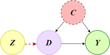
Throughout this example

\(Z\) is the instrument,
\(X\) is a vector of covariates,
\(D\) is treatment variable,
\(Y\) is the outcome.

Next, we will run a simulation, where we will generate two synthetic data sets, one where the instrument is weak and another where it is not. Then, we will compare the output of the standard way to compute confidence intervals using the DoubleMLIIVM class, with the confidence sets computed using the robust_confset() method from the same class. We will see that using the robust_confset() method is an easy way to ensure the results of an analysis are robust to weak instruments.

[1]:

import numpy as np
import pandas as pd
import random
from sklearn.base import BaseEstimator, ClassifierMixin
from sklearn.linear_model import LinearRegression, LogisticRegression
import doubleml as dml

np.random.seed(1234)
random.seed(1234)

Running a small simulation#

The following function generates data from an instrumental variables model. The true_effect argument is the estimand of interest, the true effect of the treatment on the outcome. The instrument_strength argument is a measure of the strength of the instrument. The higher it is, the stronger the correlation is between the instrument and the treatment. Notice that the instrument is fully randomized.

[2]:

def generate_weakiv_data(n_samples, true_effect, instrument_strength):
    u = np.random.normal(0, 2, size=n_samples)
    X = np.random.normal(0, 1, size=n_samples)
    Z = np.random.binomial(1, 0.5, size=n_samples)
    D = instrument_strength * Z + u
    D = np.array(D > 0, dtype=int)
    Y = true_effect * D + np.sign(u)
    return pd.DataFrame({"Y": Y, "Z": Z, "D": D, "X": X})

To fit the DML model, we need to decide on how we will estimate the nuisance functions. We will use a linear regression model for \(g\), and a logistic regression for \(r\). We will assume that we know the true \(m\) function, as is the case in a controlled experiment, such as an AB test. The following class defines defines this “fake” estimator.

[3]:

class TrueMFunction(BaseEstimator, ClassifierMixin):
    def __init__(self, prob_dist=(0.5, 0.5)):
        self.prob_dist = prob_dist

    def fit(self, X, y):
        self.prob_dist_ = np.array(self.prob_dist)
        self.classes_ = np.array(sorted(set(y)))
        return self

    def predict_proba(self, X):
        return np.tile(self.prob_dist_, (len(X), 1))

    def predict(self, X):
        return np.full(len(X), self.classes_[np.argmax(self.prob_dist_)])

We will now run a loop, where for each of \(100\) replications we will generate data using the previously defined function. We will take a sample size of \(5000\), a true effect equal to \(1\), and take two possible values for the instrument strength: \(0.003\) and \(1\). In the latter case the instrument is strong, in the former it is weak. We will then compute both the robust and the standard confidence intervals, check whether they contain the true effect, and compute their length.

[4]:

n_samples = 5000
true_effect = 1
output_list = []
for _ in range(100):
    for instrument_strength in [0.003, 1]:
        dataset = generate_weakiv_data(n_samples = n_samples, true_effect = true_effect, instrument_strength = instrument_strength)
        dml_data = dml.DoubleMLData(
            dataset, y_col='Y', d_cols='D',
            z_cols='Z', x_cols='X'
        )
        ml_g = LinearRegression()
        ml_m = TrueMFunction()
        ml_r = LogisticRegression(penalty=None)
        dml_iivm = dml.DoubleMLIIVM(dml_data, ml_g, ml_m, ml_r)
        dml_iivm.fit()
        dml_standard_ci = dml_iivm.confint(joint=False)
        dml_robust_confset = dml_iivm.robust_confset()
        dml_covers = dml_standard_ci["2.5 %"].iloc[0] <= true_effect <= dml_standard_ci["97.5 %"].iloc[0]
        robust_covers = any(interval[0] <= true_effect <= interval[1] for interval in dml_robust_confset)
        dml_length = dml_standard_ci["97.5 %"].iloc[0] - dml_standard_ci["2.5 %"].iloc[0]
        dml_robust_length = max(interval[1] - interval[0] for interval in dml_robust_confset)
        output_list.append({
            "instrument_strength": instrument_strength,
            "dml_covers": dml_covers,
            "robust_covers": robust_covers,
            "dml_length": dml_length,
            "robust_length": dml_robust_length
        })
results_df = pd.DataFrame(output_list)

Having stored the results of the simulation in the results_df dataframe, we will compute some summary statistics. We see in the table below that, when the instrument is strong, the standard DML confidence interval and the robust confidence set behave similarly, with coverage close to the nominal level and similar median lengths. On the other hand, when the instrument is strong, the coverage of the standard DML confidence interval is very low, whereas the coverage of the robust confidence set is again close to the nominal value. Note that in this case the robust confidence set has an infinite median length. When the robust confidence set has infinite length, the analyst should interpret the results as indicating that the data contains little information about the estimand of interest, possibly because the instrument is weak.

[5]:

results_df = pd.DataFrame(output_list)
summary_df = results_df.groupby("instrument_strength").agg(
    **{"DML coverage": ("dml_covers", "mean"),
       "Robust coverage": ("robust_covers", "mean"),
       "DML median length": ("dml_length", "median"),
       "Robust median length": ("robust_length", "median")}
)
print(summary_df)

                     DML coverage  Robust coverage  DML median length  \
instrument_strength
0.003                        0.15             0.91           0.489567
1.000                        0.93             0.92           0.572717

                     Robust median length
instrument_strength
0.003                                 inf
1.000                            0.582754

References#

Chernozhukov, V., Chetverikov, D., Demirer, M., Duflo, E., and Hansen, C. (2018). Double/debiased machine learning for treatment and structural parameters. The Econometrics Journal, 21(1):C1–C68.
Ma, Y. (2023). Identification-robust inference for the late with high-dimensional covariates. arXiv preprint arXiv:2302.09756.
Stock, J. H. and Wright, J. H. (2000). GMM with weak identification. Econometrica, 68(5):1055–1096.
Takatsu, K., Levis, A. W., Kennedy, E., Kelz, R., and Keele, L. (2023). Doubly robust machine learning for an instrumental variable study of surgical care for cholecystitis. arXiv preprint arXiv:2307.06269.