10. Sensitivity analysis

The DoubleML package implements sensitivity analysis with respect to omitted variable bias based on Chernozhukov et al. (2022).

10.1. General algorithm

The section Theory contains a general summary and the relevant defintions, whereas Implementation considers the general part of the implementation.

10.1.1. Theory

Assume that we can write the model in the following representation

\[\theta_0 = \mathbb{E}[m(W,g_0)],\]

where usually \(g_0(W) = \mathbb{E}[Y|X, D]\) (currently, the sensitivity analysis is only available for linear models). As long as \(\mathbb{E}[m(W,f)]\) is a continuous linear functional of \(f\), there exists a unique square integrable random variable \(\alpha_0(W)\), called Riesz representer (see Riesz-Fréchet representation theorem), such that

\[\theta_0 = \mathbb{E}[g_0(W)\alpha_0(W)].\]

The target parameter \(\theta_0\) has the following representation

\[\theta_0 = \mathbb{E}[m(W,g_0) + (Y-g_0(W))\alpha_0(W)],\]

which corresponds to a Neyman orthogonal score function (orthogonal with respect to nuisance elements \((g, \alpha)\)). To bound the omitted variable bias, the following further elements are needed. The variance of the outcome regression

\[\sigma_0^2 := \mathbb{E}[(Y-g_0(W))^2]\]

and the second moment of the Riesz representer

\[\nu_0^2 := \mathbb{E}[\alpha_0(W)^2] =2\mathbb{E}[m(W,\alpha_0)] - \mathbb{E}[\alpha_0(W)^2].\]

Both representations are Neyman orthogonal with respect to \(g\) and \(\alpha\), respectively. Further, define the corresponding score functions

\[\begin{split}\psi_{\sigma^2}(W, \sigma^2, g) &:= (Y-g_0(W))^2 - \sigma^2\\ \psi_{\nu^2}(W, \nu^2, \alpha) &:= 2m(W,\alpha) - \alpha(W)^2 - \nu^2.\end{split}\]

Recall that the parameter \(\theta_0\) is identified via the moment condition

\[\theta_0 = \mathbb{E}[m(W,g_0)].\]

If \(W=(Y, D, X)\) does not include all confounding variables, the “true” target parameter \(\tilde{\theta}_0\) would only be identified via the extendend (or “long”) form

\[\tilde{\theta}_0 = \mathbb{E}[m(\tilde{W},\tilde{g}_0)],\]

where \(\tilde{W}=(Y, D, X, A)\) includes the unobserved counfounders \(A\). In Theorem 2 of their paper Chernozhukov et al. (2022) are able to bound the omitted variable bias

\[|\tilde{\theta}_0 -\theta_0|^2 = \rho^2 B^2,\]

where

\[B^2 := \mathbb{E}\Big[\big(g(W) - \tilde{g}(\tilde{W})\big)^2\Big]\mathbb{E}\Big[\big(\alpha(W) - \tilde{\alpha}(\tilde{W})\big)^2\Big],\]

denotes the product of additional variations in the outcome regression and Riesz representer generated by omitted confounders and

\[\rho^2 := \textrm{Cor}^2\Big(g(W) - \tilde{g}(\tilde{W}),\alpha(W) - \tilde{\alpha}(\tilde{W})\Big),\]

denotes the correlations between the deviations generated by omitted confounders. The choice \(\rho=1\) is conservative and accounts for adversarial confounding. Further, the bound can be expressed as

\[B^2 := \sigma_0^2 \nu_0^2 C_Y^2 C_D^2,\]

where

\[ \begin{align}\begin{aligned}C_Y^2 &:= \frac{\mathbb{E}[(\tilde{g}(\tilde{W}) - g(W))^2]}{\mathbb{E}[(Y - g(W))^2]}\\C_D^2 &:=\frac{1 - \frac{\mathbb{E}\big[\alpha(W)^2\big]}{\mathbb{E}\big[\tilde{\alpha}(\tilde{W})^2\big]}}{\frac{\mathbb{E}\big[\alpha(W)^2\big]}{\mathbb{E}\big[\tilde{\alpha}(\tilde{W})^2\big]}}.\end{aligned}\end{align} \]

As \(\sigma_0^2\) and \(\nu_0^2\) do not depend on the unobserved confounders \(A\) they are identified. Further, the other parts have the following interpretations

• cf_y\(:=\frac{\mathbb{E}[(\tilde{g}(\tilde{W}) - g(W))^2]}{\mathbb{E}[(Y - g(W))^2]}\) measures the proportion of residual variance in the outcome \(Y\) explained by the latent confounders \(A\)

• cf_d\(:=1 - \frac{\mathbb{E}\big[\alpha(W)^2\big]}{\mathbb{E}\big[\tilde{\alpha}(\tilde{W})^2\big]}\) measures the proportion of residual variance in the Riesz representer \(\tilde{\alpha}(\tilde{W})\) generated by the latent confounders \(A\)

Note

• cf_y has the interpretation as the nonparametric partial \(R^2\) of \(A\) with \(Y\) given \((D,X)\)

\[\frac{\textrm{Var}(\mathbb{E}[Y|D,X,A]) - \textrm{Var}(\mathbb{E}[Y|D,X])}{\textrm{Var}(Y)-\textrm{Var}(\mathbb{E}[Y|D,X])}\]

• For model-specific interpretations of cf_d or \(C_D^2\), see the corresponding chapters (e.g. Partially linear regression model (PLR)).

Consequently, for given values cf_y and cf_d, we can create lower and upper bounds for target parameter \(\tilde{\theta}_0\) of the form

\[\theta_{\pm}:=\theta_0 \pm |\rho| \sigma_0 \nu_0 C_Y C_D\]

Let \(\psi(W,\theta,\eta)\) the (correctly scaled) score function for the target parameter \(\theta_0\). Then

\[\psi_{\pm}(W,\theta,\eta_\pm):= \psi(W,\theta,\eta) \pm \frac{|\rho| C_Y C_D}{2 \sigma \nu} \Big(\sigma^2 \psi_{\nu^2}(W, \nu^2, \alpha) + \nu^2 \psi_{\sigma^2}(W, \sigma^2, g)\Big)\]

determines a orthongonal score function for \(\theta_{\pm}\), with nuisance elements \(\eta_\pm:=(g, \alpha, \sigma, \nu)\). The score can be used to calculate the standard deviations of \(\theta_{\pm}\) via

\[\sigma^2_{\pm}= \mathbb{E}[\psi_{\pm}(W,\theta,\eta_\pm)^2]\]

For more detail and interpretations see Chernozhukov et al. (2022).

10.1.2. Implementation

The Partially linear regression model (PLR) will be used as an example

Python

In [1]: import numpy as np

In [2]: import doubleml as dml

In [3]: from doubleml.datasets import make_plr_CCDDHNR2018

In [4]: from sklearn.ensemble import RandomForestRegressor

In [5]: from sklearn.base import clone

In [6]: learner = RandomForestRegressor(n_estimators=100, max_features=20, max_depth=5, min_samples_leaf=2)

In [7]: ml_l = clone(learner)

In [8]: ml_m = clone(learner)

In [9]: np.random.seed(1111)

In [10]: data = make_plr_CCDDHNR2018(alpha=0.5, n_obs=500, dim_x=20, return_type='DataFrame')

In [11]: obj_dml_data = dml.DoubleMLData(data, 'y', 'd')

In [12]: dml_plr_obj = dml.DoubleMLPLR(obj_dml_data, ml_l, ml_m)

If the sensitivity analysis is implemented (see Model-specific implementations), the corresponding sensitivity elements are estimated automatically by calling the fit() method. In most cases these elements are based on the following plug-in estimators

\[ \begin{align}\begin{aligned}\hat{\sigma}^2 &:= \mathbb{E}_n[(Y-\hat{g}(W))^2]\\\hat{\nu}^2 &:= \mathbb{E}_n[2m(W,\hat{\alpha}) - \hat{\alpha}(W)^2]\end{aligned}\end{align} \]

where \(\hat{g}(W)\) and \(\hat{\alpha}(W)\) denote the cross-fitted predictions of the outcome regression and the Riesz representer (both are model specific, see Model-specific implementations). Further, the corresponding scores are defined as

\[\begin{split}\psi_{\sigma^2}(W, \hat{\sigma}^2, g) &:= (Y-\hat{g}(W))^2 - \hat{\sigma}^2\\ \psi_{\nu^2}(W, \hat{\nu}^2, \alpha) &:= 2m(W,\hat{\alpha}) - \hat{\alpha}(W)^2 - \hat{\nu}^2.\end{split}\]

After the fit() call, the sensitivity elements are stored in a dictionary and can be accessed via the sensitivity_elements property.

Python

In [13]: dml_plr_obj.fit()
Out[13]: <doubleml.double_ml_plr.DoubleMLPLR at 0x7fa68017db80>

In [14]: dml_plr_obj.sensitivity_elements.keys()
Out[14]: dict_keys(['sigma2', 'nu2', 'psi_sigma2', 'psi_nu2'])

Each value is a \(3\)-dimensional array, with the variances being of form (1, n_rep, n_coefs) and the scores of form (n_obs, n_rep, n_coefs). The sensitivity_analysis() method then computes the upper and lower bounds for the estimate, based on the sensitivity parameters cf_y, cf_d and rho (default is rho=1.0 to account for adversarial confounding). Additionally, one-sided confidence bounds are computed based on a supplied significance level (default level=0.95). The results are summarized as a formatted string in the sensitivity_summary

Python

In [15]: dml_plr_obj.sensitivity_analysis(cf_y=0.03, cf_d=0.03, rho=1.0, level=0.95)
Out[15]: <doubleml.double_ml_plr.DoubleMLPLR at 0x7fa68017db80>

In [16]: print(dml_plr_obj.sensitivity_summary)
================== Sensitivity Analysis ==================

------------------ Scenario          ------------------
Significance Level: level=0.95
Sensitivity parameters: cf_y=0.03; cf_d=0.03, rho=1.0

------------------ Bounds with CI    ------------------
   CI lower  theta lower     theta  theta upper  CI upper
d  0.410112     0.484032  0.514216     0.544399  0.618163

------------------ Robustness Values ------------------
   H_0     RV (%)    RVa (%)
d  0.0  40.147026  35.207071

or can be directly accessed via the sensitivity_params property.

Python

In [17]: dml_plr_obj.sensitivity_params
Out[17]: 
{'theta': {'lower': array([0.48403222]), 'upper': array([0.54439924])},
 'se': {'lower': array([0.04494057]), 'upper': array([0.04484505])},
 'ci': {'lower': array([0.41011156]), 'upper': array([0.61816278])},
 'rv': array([0.40147026]),
 'rva': array([0.35207071]),
 'input': {'cf_y': 0.03,
  'cf_d': 0.03,
  'rho': 1.0,
  'level': 0.95,
  'null_hypothesis': array([0.])}}

The bounds are saved as a nested dictionary, where the keys 'theta' denote the bounds on the parameter \(\hat{\theta}_{\pm}\), 'se' denotes the corresponding standard error and 'ci' denotes the lower and upper confidence bounds for \(\hat{\theta}_{\pm}\). Each of the keys refers to a dictionary with keys 'lower' and 'upper' which refer to the lower or upper bound, e.g. sensitivity_params['theta']['lower'] refers to the lower bound \(\hat{\theta}_{-}\) of the estimated cofficient .

Further, the sensitivity analysis has an input parameter theta (with default theta=0.0), which refers to the null hypothesis used for each coefficient. This null hypothesis is used to calculate the robustness values as displayed in the sensitivity_params.

The robustness value $RV$ is defined as the required confounding strength (cf_y=rv and cf_d=rv), such that the lower or upper bound of the causal parameter includes the null hypothesis. If the estimated parameter \(\hat{\theta}\) is larger than the null hypothesis the lower bound is used and vice versa. The robustness value $RVa$ defined analogous, but additionally incorporates statistical uncertainty (as it is based on the confidence intervals of the bounds).

To obtain a more complete overview over the sensitivity one can call the sensitivity_plot() method. The methods creates a contour plot, which calculates estimate of the upper or lower bound for \(\theta\) (based on the null hypothesis) for each combination of cf_y and cf_d in a grid of values.

Contour plot example (see Examples)

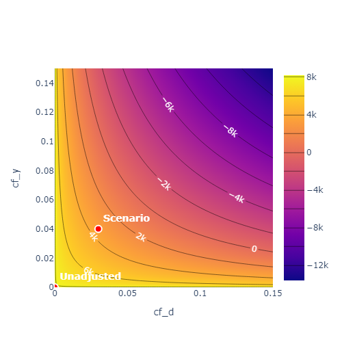
By adjusting the parameter value='ci' in the sensitivity_plot() method the bounds are displayed for the corresponding confidence level.

Note

• The sensitivity_plot() requires to call sensitivity_analysis first, since the choice of the bound (upper or lower) is based on the corresponding null hypothesis. Further, the parameters rho and level are used. Both are contained in the sensitivity_params property.

• The sensitivity_plot() is created for the first treatment variable. This can be changed via the idx_treatment parameter.

• The robustness values are given via the intersection countour of the null hypothesis and the identity.

10.1.3. Benchmarking

The input parameters for the sensitivity analysis are quite hard to interpret (depending on the model). Consequently it is challenging to come up with reasonable bounds for the confounding strength cf_y and cf_d (and rho). To get a grasp on the magnitude of the bounds a popular approach is to rely on observed confounders to obtain an informed guess on the strength of possibly unobserved confounders.

The underlying principle is relatively simple. If we have an observed confounder \(X_1\), we are able to emulate omitted confounding by purposely omitting \(X_1\) and refitting the whole model. This enables us to compare the “long” and “short” form with and without omitted confounding. Considering the sensitivity_params of both models one can estimate the corresponding strength of confounding cf_y and cf_d (and rho).

Note

• The benchmarking can also be done with a set of benchmarking variables (e.g. \(X_1, X_2, X_3\)), which tries to emulate the effect of multiple unobserved confounders.

• The approach is quite computationally demanding, as the short model that omits the benchmark variables has to be fitted.

The sensitivity_benchmark() method implements this approach. The method just requires a set of valid covariates, the benchmarking_set, to compute the benchmark. The benchmark variables have to be a subset of the covariates used in the main analysis.

Python

In [18]: dml_plr_obj.sensitivity_benchmark(benchmarking_set=["X1"])
Out[18]: 
       cf_y     cf_d      rho  delta_theta
d  0.026842  0.45688  0.97978     0.089075

The method returns a pandas.DataFrame, containing the benchmarked values for cf_y, cf_d, rho and the change in the estimates delta_theta.

Note

• The benchmarking results should be used to get an idea of the magnitude/validity of proposed confounding strength of the omitted confounders. Whether these values are close to the real confounding, depends entirely on the setting and choice of the benchmarking variables. A good benchmarking set has a strong justification which refers to the omitted confounders.

• If the benchmarking variables are only weak confounders, the estimates of rho can be slightly unstable (due to small denominators).

The implementation is based on Chernozhukov et al. (2022) Appendix D and corresponds to a generalization of the benchmarking process in the Sensemakr package for regression models to the use with double machine learning. For an introduction to Sensemakr see Cinelli and Hazlett (2020) and the Sensemakr introduction.

The benchmarked estimates are the following:

Let the subscript \(short\), denote the “short” form of the model, where the benchmarking variables are omitted.

• \(\hat{\sigma}^2_{short}\) denotes the variance of the outcome regression in the “short” form.

• \(\hat{\nu}^2_{short}\) denotes the second moment of the Riesz representer in the “short” form.

Both parameters are contained in the sensitivity_params of the “short” form. This enables the following estimation of the nonparametric \(R^2\)’s of the outcome regression

• \(\hat{R}^2:= 1 - \frac{\hat{\sigma}^2}{\textrm{Var}(Y)}\)

• \(\hat{R}^2_{short}:= 1 - \frac{\hat{\sigma}^2_{short}}{\textrm{Var}(Y)}\)

and the correlation ratio of the estimated Riesz representations

\[\hat{R}^2_{\alpha}:= \frac{\hat{\nu}^2_{short}}{\hat{\nu}^2}.\]

The benchmarked estimates are then defined as

• cf_y\(:=\frac{\hat{R}^2 - \hat{R}^2_{short}}{1 - \hat{R}^2}\) measures the proportion of residual variance in the outcome \(Y\) explained by adding the purposely omitted benchmarking_set

• cf_d\(:=\frac{1 - \hat{R}^2_{\alpha}}{\hat{R}^2_{\alpha}}\) measures the proportional gain in variation that the benchmarking_set creates in the Riesz representer

Further, the degree of adversity \(\rho\) can be estimated via

\[\hat{\rho} := \frac{\hat{\theta}_{short} - \hat{\theta}}{ \sqrt{(\hat{\sigma}^2_{short} - \hat{\sigma}^2)(\hat{\nu}^2 - \hat{\nu}^2_{short})}}.\]

For a more detailed description, see Chernozhukov et al. (2022) Appendix D.

Note

• As benchmarking requires the estimation of a seperate model, the use with external predictions is generally not possible.

10.2. Model-specific implementations

This section contains the implementation details for each specific model and model specific interpretations.

10.2.1. Partially linear regression model (PLR)

In the Partially linear regression model (PLR) the confounding strength cf_d can be further be simplified to match the explanation of cf_y. Given the that the Riesz representer takes the following form

\[ \begin{align}\begin{aligned}\alpha(W) = \frac{D-\mathbb{E}[D|X]}{\mathbb{E}[(D-\mathbb{E}[D|X]^2)]}\\\tilde{\alpha}(\tilde{W}) = \frac{D-\mathbb{E}[D|X,A]}{\mathbb{E}[(D-\mathbb{E}[D|X,A]^2)]}\end{aligned}\end{align} \]

one can show that

\[C_D^2 :=\frac{\frac{\mathbb{E}\big[\big(\mathbb{E}[D|X,A] - \mathbb{E}[D|X]\big)^2\big]}{\mathbb{E}\big[\big(D - \mathbb{E}[D|X]\big)^2\big]}}{1-\frac{\mathbb{E}\big[\big(\mathbb{E}[D|X,A] - \mathbb{E}[D|X]\big)^2\big]}{\mathbb{E}\big[\big(D - \mathbb{E}[D|X]\big)^2\big]}}.\]

Therefore,

• cf_y\(:=\frac{\mathbb{E}[(\tilde{g}(\tilde{W}) - g(W))^2]}{\mathbb{E}[(Y - g(W))^2]}\) measures the proportion of residual variance in the outcome \(Y\) explained by the latent confounders \(A\)

• cf_d\(:=\frac{\mathbb{E}\big[\big(\mathbb{E}[D|X,A] - \mathbb{E}[D|X]\big)^2\big]}{\mathbb{E}\big[\big(D - \mathbb{E}[D|X]\big)^2\big]}\) measures the proportion of residual variance in the treatment \(D\) explained by the latent confounders \(A\)

Note

In the Partially linear regression model (PLR), both cf_y and cf_d can be interpreted as nonparametric partial \(R^2\)

• cf_y has the interpretation as the nonparametric partial \(R^2\) of \(A\) with \(Y\) given \((D,X)\)

\[\frac{\textrm{Var}(\mathbb{E}[Y|D,X,A]) - \textrm{Var}(\mathbb{E}[Y|D,X])}{\textrm{Var}(Y)-\textrm{Var}(\mathbb{E}[Y|D,X])}\]

• cf_d has the interpretation as the nonparametric partial \(R^2\) of \(A\) with \(D\) given \(X\)

\[\frac{\textrm{Var}(\mathbb{E}[D|X,A]) - \textrm{Var}(\mathbb{E}[D|X])}{\textrm{Var}(D)-\textrm{Var}(\mathbb{E}[D|X])}\]

Using the partially linear regression model with score='partialling out' the nuisance_elements are implemented in the following form

\[ \begin{align}\begin{aligned}\hat{\sigma}^2 &:= \mathbb{E}_n\Big[\big(Y-\hat{l}(X) - \hat{\theta}(D-\hat{m}(X))\big)^2\Big]\\\hat{\nu}^2 &:= \mathbb{E}_n[\hat{\alpha}(W)^2] = \frac{1}{\mathbb{E}_n\big[(D - \hat{m}(X))^2\big]}\end{aligned}\end{align} \]

with scores

\[ \begin{align}\begin{aligned}\psi_{\sigma^2}(W, \hat{\sigma}^2, g) &:= \big(Y-\hat{l}(X) - \hat{\theta}(D-\hat{m}(X))\big)^2 - \hat{\sigma}^2\\\psi_{\nu^2}(W, \hat{\nu}^2, \alpha) &:= \hat{\nu}^2 - \big(D-\hat{m}(X)\big)^2\big(\hat{\nu}^2)^2.\end{aligned}\end{align} \]

If score='IV-type' the senstivity elements are instead set to

\[ \begin{align}\begin{aligned}\hat{\sigma}^2 &:= \mathbb{E}_n\Big[\big(Y - \hat{\theta}D - \hat{g}(X)\big)^2\Big]\\\psi_{\sigma^2}(W, \hat{\sigma}^2, g) &:= \big(Y - \hat{\theta}D - \hat{g}(X)\big)^2 - \hat{\sigma}^2.\end{aligned}\end{align} \]

10.2.2. Interactive regression model (IRM)

In the Interactive regression model (IRM) the target parameter can be written as

\[\theta_0 = \mathbb{E}[(g_0(1,X) - g_0(0,X))\omega(Y,D,X)]\]

where \(\omega(D,X)\) are weights (e.g. set to \(1\) for the ATE). This implies the following representations

\[ \begin{align}\begin{aligned}m(W,g) &= \big(g(1,X) - g(0,X))\omega(Y,D,X)\\\alpha(W) &= \bigg(\frac{D}{m(X)} - \frac{1-D}{1-m(X)}\bigg) \mathbb{E}[\omega(Y,D,X)|X].\end{aligned}\end{align} \]

Note

In the Interactive regression model (IRM) with for the ATE (weights equal to \(1\)), the form and interpretation of cf_y is the same as in the Partially linear regression model (PLR).

• cf_y has the interpretation as the nonparametric partial \(R^2\) of \(A\) with \(Y\) given \((D,X)\)

\[\frac{\textrm{Var}(\mathbb{E}[Y|D,X,A]) - \textrm{Var}(\mathbb{E}[Y|D,X])}{\textrm{Var}(Y)-\textrm{Var}(\mathbb{E}[Y|D,X])}\]

• cf_d takes the following form

\[\small{\frac{\mathbb{E}\Big[\big(P(D=1|X,A)(1-P(D=1|X,A))\big)^{-1}\Big] - \mathbb{E}\Big[\big(P(D=1|X)(1-P(D=1|X))\big)^{-1}\Big]}{\mathbb{E}\Big[\big(P(D=1|X,A)(1-P(D=1|X,A))\big)^{-1}\Big]}}\]

where the numerator measures the gain in average conditional precision to predict \(D\) by using \(A\) in addition to \(X\). The denominator is the average conditional precision to predict \(D\) by using \(A\) and \(X\). Consequently cf_d measures the relative gain in average conditional precision.

Remark that \(P(D=1|X,A)(1-P(D=1|X,A))\) denotes the variance of the conditional distribution of \(D\) given \((X,A)\), such that the inverse measures the precision of predicting \(D\) conditional on \((X,A)\).

Since \(C_D^2=\frac{cf_d}{1 - cf_d}\), this corresponds to

\[C_D^2= \small{\frac{\mathbb{E}\Big[\big(P(D=1|X,A)(1-P(D=1|X,A))\big)^{-1}\Big] - \mathbb{E}\Big[\big(P(D=1|X)(1-P(D=1|X))\big)^{-1}\Big]}{\mathbb{E}\Big[\big(P(D=1|X)(1-P(D=1|X))\big)^{-1}\Big]}}\]

which has the same numerator but is instead relative to the average conditional precision to predict \(D\) by using only \(X\).

Including weights changes only the definition of cf_d to

\[\frac{\mathbb{E}\left[\frac{\mathbb{E}[\omega(Y,D,X)|X,A]^2}{P(D=1|X,A)(1-P(D=1|X,A))}\right] - \mathbb{E}\left[\frac{\mathbb{E}[\omega(Y,D,X)|X]^2}{P(D=1|X)(1-P(D=1|X))}\right]}{\mathbb{E}\left[\frac{\mathbb{E}[\omega(Y,D,X)|X,A]^2}{P(D=1|X,A)(1-P(D=1|X,A))}\right]}\]

which has a interpretation as the relative weighted gain in average conditional precision.

The nuisance_elements are then computed with plug-in versions according to the general Implementation. For score='ATE', the weights are set to one

\[\omega(Y,D,X) = 1,\]

wheras for score='ATTE'

\[\omega(Y,D,X) = \frac{D}{\mathbb{E}[D]},\]

such that

\[\mathbb{E}[\omega(Y,D,X)|X] = \frac{m(X)}{\mathbb{E}[D]}.\]

10.2.3. Difference-in-Differences for Panel Data

In the Panel data with score='observational' and in_sample_normalization=True the score function implies the following representations

\[ \begin{align}\begin{aligned}m(W,g) &= \big(g(1,X) - g(0,X))\frac{D}{\mathbb{E}[D]}\\\alpha(W) &= \frac{D}{\mathbb{E}[D]} - \frac{\frac{m(X)(1-D)}{1-m(X)}}{\mathbb{E}\left[\frac{m(X)(1-D)}{1-m(X)}\right]}.\end{aligned}\end{align} \]

If instead in_sample_normalization=False, the Riesz representer changes to

\[\alpha(W) = \frac{D}{\mathbb{E}[D]} - \frac{m(X)(1-D)}{\mathbb{E}[D](1-m(X))}.\]

For score='experimental' implies the score function implies the following representations

\[ \begin{align}\begin{aligned}m(W,g) &= g(1,X) - g(0,X)\\\alpha(W) &= \frac{D}{\mathbb{E}[D]} - \frac{1-D}{1-\mathbb{E}[D]}.\end{aligned}\end{align} \]

The nuisance_elements are then computed with plug-in versions according to the general Implementation.

10.2.4. Difference-in-Differences for repeated cross-sections

In the Repeated cross-sections with score='observational' and in_sample_normalization=True the score function implies the following representations

\[ \begin{align}\begin{aligned}m(W,g) &= \Big(\big(g(1,1,X) - g(1,0,X)\big) - \big(g(0,1,X) - g(0,0,X)\big)\Big) \frac{D}{\mathbb{E}[D]}\\\alpha(W) &= \frac{DT}{\mathbb{E}[DT]} - \frac{D(1-T)}{\mathbb{E}[D(1-T)]}\\&\quad - \frac{m(X)(1-D)T}{1-m(X)}\mathbb{E}\left[\frac{m(X)(1-D)T}{1-m(X)}\right]^{-1}\\&\quad + \frac{m(X)(1-D)(1-T)}{1-m(X)}\mathbb{E}\left[\frac{m(X)(1-D)(1-T)}{1-m(X)}\right]^{-1}.\end{aligned}\end{align} \]

If instead in_sample_normalization=False, the Riesz representer (after simplifications) changes to

\[\alpha(W) = \left(\frac{T}{\mathbb{E}[D]\mathbb{E}[T]} + \frac{1-T}{\mathbb{E}[D](1-\mathbb{E}[T])}\right)\left(D - (1-D)\frac{m(X)}{1-m(X)}\right).\]

For score='experimental' and in_sample_normalization=True implies the score function implies the following representations

\[ \begin{align}\begin{aligned}m(W,g) &= \big(g(1,1,X) - g(1,0,X)\big) - \big(g(0,1,X) - g(0,0,X)\big)\\\alpha(W) &= \frac{DT}{\mathbb{E}[DT]} - \frac{D(1-T)}{\mathbb{E}[D(1-T)]} - \frac{(1-D)T}{\mathbb{E}[(1-D)T]} + \frac{(1-D)(1-T)}{\mathbb{E}[(1-D)(1-T)]}.\end{aligned}\end{align} \]

And again, if instead in_sample_normalization=False, the Riesz representer (after simplifications) changes to

\[\alpha(W) = \frac{DT}{\mathbb{E}[D]\mathbb{E}[T]} - \frac{D(1-T)}{\mathbb{E}[D](1-\mathbb{E}[T])} - \frac{(1-D)T}{(1-\mathbb{E}[D])\mathbb{E}[T]} + \frac{(1-D)(1-T)}{(1-\mathbb{E}[D])(1-\mathbb{E}[T])}.\]

The nuisance_elements are then computed with plug-in versions according to the general Implementation.