DoubleML - Sensitivity Analysis

Tools for Causality
Grenoble, Sept 25 - 29, 2023
Philipp Bach, Sven Klaassen

Motivation: Sensitivity Analysis

Motivation: DoubleML Workflow

0. Problem Formulation

1. Data-Backend

2. Causal Model

3. ML Methods

4. DML Specification

5. Estimation

6. Inference

7. Sensitivity Analysis

• Earlier we introduced 6 steps of the DoubleML workflow.

• Actually, there is a 7th step that is often overlooked: Sensitivity Analysis

Motivation

• Whenever we have (properly collected) experimental data, we have good reason to believe that the independence assumption holds, i.e., the treatment assignment is independent of the potential outcomes

\[ Y(d) ⊥ D \]

• However, what about causal evidence from observational data? 😱

“A well designed RCT is the dream of any scientist”, Source: Chapter 2 of Facure and Germano (2021)

Motivation

• Observational studies are often based on the assumption of conditional independence¹

• Conditional on pre-treatment confounders \(X\), the treatment is as good as randomly assigned

\[ Y(d) ⊥ D \mid X \]

• In general, the independence assumption is not testable!

Code

import networkx as nx
import matplotlib.pyplot as plt

G = nx.DiGraph()

# Add nodes
G.add_node("D")
G.add_node("Y")
G.add_node("X")
G.add_edge("D", "Y")
G.add_edge("X", "Y")
G.add_edge("X", "D")

# Draw the graph
plt.figure(figsize=(4, 3)) 
pos = {"D": (0, 0), "Y": (2, 0), "X": (1,1)}
edge_colors = ['black', 'black', 'black']
nx.draw(G, pos, with_labels=True, node_size=800, node_color='lightblue',
 edge_color=edge_colors)
plt.show()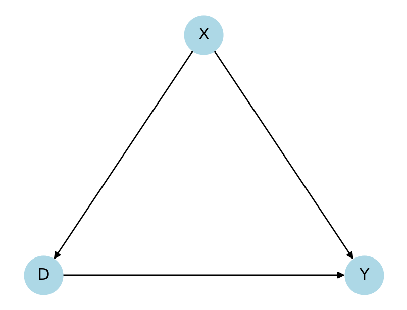

DAG: Causal Effect of D on Y, with observed confounders X.

1. Also known as conditional exogeneity, unconfoundedness or ignorability

Motivation

• What if the conditional independence assumption is violated?

• Unobserved confounders U would introduce an omitted variable bias/ selection-into-treatment bias

• Key questions:

1. How strong would a confounding relationship need to be in order to change the conclusions of our analysis?

2. Would such a confounding relationship be plausibly present in our data?

Code

import networkx as nx
import matplotlib.pyplot as plt

G = nx.DiGraph()

# Add nodes
G.add_node("D")
G.add_node("Y")
G.add_node("X")
G.add_node("U")
G.add_edge("D", "Y")
G.add_edge("X", "Y")
G.add_edge("X", "D")
G.add_edge("U", "D")
G.add_edge("U", "Y")

# Draw the graph
plt.figure(figsize=(4, 3)) 
pos = {"D": (0, 0), "Y": (2, 0), "X": (1,1), "U": (1,-1)}
edge_colors = ['black', 'black', 'black', 'red', 'blue']
nx.draw(G, pos, with_labels=True, node_size=800, node_color='lightblue',
 edge_color=edge_colors)
plt.show()

DAG: Causal Effect of D on Y, with observed confounders X and unobserved confounders U.

Outlook: Sensitivity Analysis

1. How strong would a confounding relationship need to be in order to change the conclusions of our analysis?

• Model the strength of the confounding relationships in terms of some sensitivity parameters, i.e.,
  • \(U\) \(\rightarrow\) \(D\) and
  • \(U\) \(\rightarrow\) \(Y\)

2. Would such a confounding relationship be plausibly present in our data?

• Benchmarking framework

Code

import networkx as nx
import matplotlib.pyplot as plt

G = nx.DiGraph()

# Add nodes
G.add_node("D")
G.add_node("Y")
G.add_node("X")
G.add_node("U")
G.add_edge("D", "Y")
G.add_edge("X", "Y")
G.add_edge("X", "D")
G.add_edge("U", "D")
G.add_edge("U", "Y")

# Draw the graph
plt.figure(figsize=(4, 3)) 
pos = {"D": (0, 0), "Y": (2, 0), "X": (1,1), "U": (1,-1)}
edge_colors = ['black', 'black', 'black', 'red', 'blue']
nx.draw(G, pos, with_labels=True, node_size=800, node_color='lightblue',
 edge_color=edge_colors)
plt.show()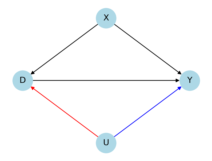

DAG: Causal Effect of D on Y, with observed confounders X and unobserved confounders U.

Example: Linear Regression Model

Consider a linear regression model with observed and unobserved confounders \(X\) and \(U\), respectively

\[ \begin{align*} Y &= \theta_0 D + \beta X + \gamma_1 U + \epsilon,\\ D &= \delta X + \gamma_2 U + \nu, \end{align*} \] with \(\epsilon\) and \(\nu\) being uncorrelated error terms and \(\theta_0\) corresponds to the average treatment effect of the (continuous) treatment \(D\) on \(Y\).

• Short parameter \(\theta_{0,s}\) - corresponds to model using data \(\{Y, D, X\}\) (short model)¹

• Long parameter \(\theta_0\) - corresponds to model using data \(\{Y, D, X, U\}\) (long model)

\(\Rightarrow\) Omitted variable bias:

\[ \theta_{0,s} - \theta_{0} \]

1. Reference: Chernozhukov et al. (2022)

Example: Linear Regression Model

\[ \begin{align*} Y &= \theta D + \beta X + \gamma_1 U + \epsilon,\\ D &= \delta X + \gamma_2 U + \nu, \end{align*} \]

• Simple idea for sensitivity analysis:
  • Parametrically model / simulate the unobserved confounder \(U\) and derive sensitivity bounds according to different values of \(\gamma_1\) and \(\gamma_2\)
  • ⚡ Problem: Sensitivity results will depend on the parametric model for \(U\), which might be too simplistic, for example,
    • Binary or continuous \(U\)?
    • Single or multiple confounders \(U\)?
    • Correlation of \(U\) with \(X\)?

• Alternative: Use \(R^2\)-based sensitivity parameters (Cinelli and Hazlett 2020)

Example: Linear Regression Model

Sensitivity parameters in Cinelli and Hazlett (2020)

• \(U\) \(\rightarrow\) \(D\): Share of residual variation of \(D\) explained by omitted confounder(s) \(U\), after taking \(X\) into account, \(R^2_{D\sim U|X}\)

• \(U\) \(\rightarrow\) \(Y\): Share of residual variation of \(Y\) explained by \(U\), after taking \(X\) and \(D\) into account, \(R^2_{Y\sim U|D,X}\)

Code

import networkx as nx
import matplotlib.pyplot as plt

G = nx.DiGraph()

# Add nodes
G.add_node("D")
G.add_node("Y")
G.add_node("X")
G.add_node("U")
G.add_edge("D", "Y")
G.add_edge("X", "Y")
G.add_edge("X", "D")
G.add_edge("U", "D")
G.add_edge("U", "Y")

# Draw the graph
plt.figure(figsize=(4, 3)) 
pos = {"D": (0, 0), "Y": (2, 0), "X": (1,1), "U": (1,-1)}
edge_colors = ['black', 'black', 'black', 'red', 'blue']
nx.draw(G, pos, with_labels=True, node_size=800, node_color='lightblue',
 edge_color=edge_colors)
plt.show()

DAG: Causal Effect of D on Y, with observed confounders X and unobserved confounders U.

Example: Linear Regression Model

Results in Cinelli and Hazlett (2020)

• Bounds for the omitted variable bias \(\theta_{0,s} - \theta_{0}\) and confidence intervals as based on values for these sensitivity parameters

• Various measures to be reported:

  • Robustness value
  • Extreme scenarios

• Visualization:

  • Contour plots (Imbens 2003)

Example contour plot, Source DoubleML User Guide

Example: Linear Regression Model

• The approach by Cinelli and Hazlett (2020) can be used to derive sensitivity bounds depending on various specifications of the sensitivity parameters

• However, how do we know if the values for these parameters are plausible?

• Cinelli and Hazlett (2020) also develop a formal benchmarking framework to relate the values of the sensitivity parameters to observed confounders

• Idea:

  • Mimic omitting an important observed (benchmark) confounder and re-compute the values of the sensitivity parameters
  • Use domain expertise to assess plausibility of the confounding scenarios

Example: Linear Regression Model

Benchmarking example

• Assume we know that \(X_1\) is a very important predictor for \(Y\) and \(D\), then we can calculate the benchmark values for the sensitivity parameters, i.e.,

  • \(X_1\) \(\rightarrow\) \(D\): Share of residual variation of \(D\) explained by the omitted confounder(s) \(X_1\), after taking \(X_{-1}\)into account,¹ \(R^2_{D\sim X_1|X_{-1}}\)

  • \(X_1\) \(\rightarrow\) \(Y\): Share of residual variation of \(Y\) explained by \(X_1\), after taking \(X_{-1}\) and \(D\) into account, \(R^2_{Y\sim X_1|D,X_{-1}}\)

• Given the values for the benchmarking variable, we can judge whether critical values of the sensitivity parameters are plausible or not

1. \(X_{-1}\) denotes the set of all predictors except \(X_1\)

Sensitivity Analysis for Causal ML

Sensitivity Analysis for Causal ML

• The framework of Cinelli and Hazlett (2020) is very intuitive and powerful for the linear regression model

• Here, linearity helps to endow the sensitivity parameters with an intuitive interpretation (partial \(R^2\) )

• However, the framework itself does not directly expand to non-linear models, such as the interactive regression model

Sensitivity Analysis for Causal ML

• Chernozhukov et al. (2022) propose a generalization of the sensitivity analysis framework to non-linear models and is suitable for ML-based estimation

• We do not go into the formal details¹ as the approach is technically evolved

• We sketch the main ideas and demonstrate the implementation in DoubleML with an example

1. See the summary in the DoubleML User Guide and the paper by Chernozhukov et al. (2022) for details

Sensitivity Analysis for Causal ML

• The sensitivity parameters in Cinelli and Hazlett (2020) are formulated in terms of partial \(R^2\) measures which apply to linear relationships

• However, we might want to model non-linear relationships

• Example: Partially linear regression model

\[ \begin{align}\begin{aligned}Y = D \theta_0 + g_0(X) + \zeta, & &\mathbb{E}(\zeta | D,X) = 0,\\D = m_0(X) + V, & &\mathbb{E}(V | X) = 0,\end{aligned}\end{align} \] with nonlinear functions \(g_0\) and \(m_0\).

• Moreover, we would like to apply sensitivity analysis for
  • Other causal models, such as the interactive regression model
  • ML-based estimation

Sensitivity Analysis for Causal ML

Brief summary: Chernozhukov et al. (2022)

• Generalization of the ideas in Cinelli and Hazlett (2020) to a broad class of causal models, including

  • Partially linear regression
  • Interactive regression model
  • Difference-in-Differences

• The approach is based on the so-called Riesz-Fréchet representation, which is related to the orthogonal score of a causal model (debiasing)

• Sensitivity parameters are defined in terms of nonparametric partial \(R^2\)

Sensitivity Analysis for Causal ML

Brief summary: Chernozhukov et al. (2022)

Advantages

• Various causal models (including non-separable models, like IRM)

• ML-based estimation

• Non-linear confounding relationships

Limitations

• Technical complexity

• Generalization comes at costs of interpretability (\(R^2\)?)

Sensitivity Analysis in DoubleML

Sensitivity Analysis in DoubleML

• Let’s complete the 7th step of the DoubleML workflow example¹

• We obtained the following results for the ATE (IRM)

dml_irm_rf.summary.round(3)

	coef	std err	t	P>|t|	2.5 %	97.5 %
e401	8121.565	1106.553	7.34	0.0	5952.76	10290.369

• Now, we wonder how robust these effects are with respect to unobserved confounding

1. You can find an online version here

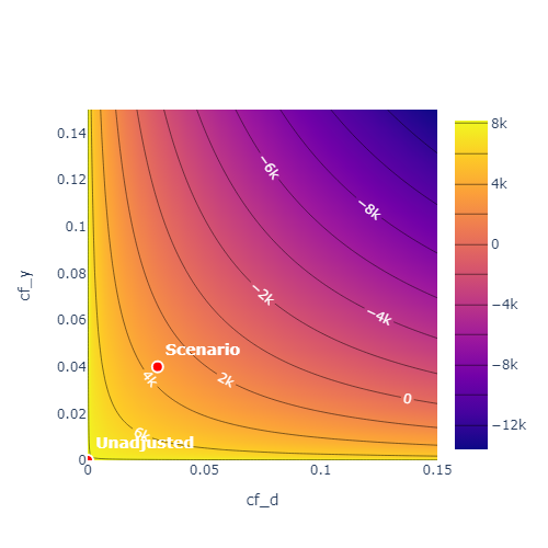
Sensitivity Analysis in DoubleML

• At given values for the sensitivity parameters cf_d and cf_y, we can compute bounds for
  • The parameter \(\theta_0\) and
  • \((1-\alpha)\) confidence intervals
• The interpretation of the sensitivity parameters depends on the causal model

PLR

• \(U\) \(\rightarrow\) \(D\): Partial nonparametric \(R^2\) of \(U\) with \(D\), given \(X\)
• \(U\) \(\rightarrow\) \(Y\): Partial nonparametric \(R^2\) of \(U\) with \(Y\), given \(D\) and \(X\)

Code

import networkx as nx
import matplotlib.pyplot as plt

G = nx.DiGraph()

# Add nodes
G.add_node("D")
G.add_node("Y")
G.add_node("X")
G.add_node("U")
G.add_edge("D", "Y")
G.add_edge("X", "Y")
G.add_edge("X", "D")
G.add_edge("U", "D")
G.add_edge("U", "Y")

# Draw the graph
plt.figure(figsize=(4, 3)) 
pos = {"D": (0, 0), "Y": (2, 0), "X": (1,1), "U": (1,-1)}
edge_colors = ['black', 'black', 'black', 'red', 'blue']
nx.draw(G, pos, with_labels=True, node_size=800, node_color='lightblue',
 edge_color=edge_colors)
plt.show()

DAG: Causal Effect of D on Y, with observed confounders X and unobserved confounders U.

Sensitivity Analysis in DoubleML

• At given values for the sensitivity parameters cf_d and cf_y, we can compute bounds for
  • The parameter \(\theta_0\) and
  • \((1-\alpha)\) confidence intervals
• The interpretation of the sensitivity parameters depends on the causal model

IRM

• \(U\) \(\rightarrow\) \(D\): Average gain in quality to predict \(D\) by using \(U\) in addition to \(X\) (relative)
• \(U\) \(\rightarrow\) \(Y\): Partial nonparametric \(R^2\) of \(U\) with \(Y\), given \(D\) and \(X\)

Code

import networkx as nx
import matplotlib.pyplot as plt

G = nx.DiGraph()

# Add nodes
G.add_node("D")
G.add_node("Y")
G.add_node("X")
G.add_node("U")
G.add_edge("D", "Y")
G.add_edge("X", "Y")
G.add_edge("X", "D")
G.add_edge("U", "D")
G.add_edge("U", "Y")

# Draw the graph
plt.figure(figsize=(4, 3)) 
pos = {"D": (0, 0), "Y": (2, 0), "X": (1,1), "U": (1,-1)}
edge_colors = ['black', 'black', 'black', 'red', 'blue']
nx.draw(G, pos, with_labels=True, node_size=800, node_color='lightblue',
 edge_color=edge_colors)
plt.show()

DAG: Causal Effect of D on Y, with observed confounders X and unobserved confounders U.

Sensitivity Analysis in DoubleML

• Sensitivity analysis as of Chernozhukov et al. (2022) is implementented in the method sensitivity_analysis()

dml_irm_rf.sensitivity_analysis()
print(dml_irm_rf.sensitivity_summary)

================== Sensitivity Analysis ==================

------------------ Scenario          ------------------
Significance Level: level=0.95
Sensitivity parameters: cf_y=0.03; cf_d=0.03, rho=1.0

------------------ Bounds with CI    ------------------
        CI lower  theta lower        theta   theta upper      CI upper
e401  2145.47168  4033.019801  8121.564764  12210.109726  14101.927365

------------------ Robustness Values ------------------
      H_0    RV (%)   RVa (%)
e401  0.0  5.870442  4.478475

• Robustness value RV: Minimum strength of the confounding relationship that would lead to an adjustment of the parameter bounds such that they include \(0\)¹

• A confounding relationship with cf_d\(=\)cf_y\(=5.87\%\) would suffice to set the lower bound for the ATE to \(0\)

1. It is also possible to choose another hypothesized value \(\theta \neq 0\)

Sensitivity Analysis in DoubleML

• Sensitivity analysis as of Chernozhukov et al. (2022) is implementented in the method sensitivity_analysis()

dml_irm_rf.sensitivity_analysis()
print(dml_irm_rf.sensitivity_summary)

================== Sensitivity Analysis ==================

------------------ Scenario          ------------------
Significance Level: level=0.95
Sensitivity parameters: cf_y=0.03; cf_d=0.03, rho=1.0

------------------ Bounds with CI    ------------------
        CI lower  theta lower        theta   theta upper      CI upper
e401  2145.47168  4033.019801  8121.564764  12210.109726  14101.927365

------------------ Robustness Values ------------------
      H_0    RV (%)   RVa (%)
e401  0.0  5.870442  4.478475

• Robustness value RVa: Minimum strength of the confounding relationship that would lead to an adjustment of the (1-\(\alpha\)) confidence interval bounds such that they intersect with \(0\)

• A confounding relationship with cf_d\(=\)cf_y\(=4.48\%\) would suffice to let the lower bound for the \(95\%\) confidence interval include \(0\) (=render effect non-significant)

Sensitivity Analysis in DoubleML

Visualization

• Contour plots make it possible to visualize many different sensitivity scenarios at once

• Each contour line indicates the combinations of cf_d and cf_y that lead to the same level of bias

dml_irm_rf.sensitivity_plot()

Sensitivity Analysis in DoubleML

• So far, we considered how we can perform sensitivity analysis for a given set of parameter values

• However, we might wonder how we can choose plausible values for the sensitivity parameters

• There are basically two ways to do this:

  1. Domain expertise: Use domain expertise to postulate certain values for the confounding scenarios
  2. Benchmarking: Mimic omitting an important observed (benchmark) confounder and re-compute the values of the sensitivity parameters

Sensitivity Analysis in DoubleML

Benchmarking

• We consider the variable inc which measures individuals’ income

• For more details, see Chapter 6 in Chernozhukov et al. (2022) as well as the notebook in the DoubleML Example Gallery

benchmark_inc = dml_irm_rf.sensitivity_benchmark(benchmarking_set=["inc"])
print(benchmark_inc)

          cf_y      cf_d       rho  delta_theta
e401  0.145986  0.175333  0.211203  4183.495564

Sensitivity Analysis in DoubleML

Benchmarking

• Let’s add this scenario to the contour plot

benchmark_dict = {"cf_y" : [benchmark_inc.loc["e401", "cf_y"]],
                  "cf_d" : [benchmark_inc.loc["e401", "cf_d"]],
                  "name" : ["inc"]}
dml_irm_rf.sensitivity_plot(benchmarks=benchmark_dict, grid_bounds=(0.23, 0.23))

Sensitivity Analysis in DoubleML

Degree of adversity

• When specifying the main confounding scenario in the sensitivity_analysis() call, there is a parameter called \(\rho\) (degree of adversity)

• Informally speaking, \(\rho \in [-1, 1]\) measures the correlation between the deviations that are created by the confounder(s) in terms of the relationships

  • \(U\) \(\rightarrow\) \(D\) and
  • \(U\) \(\rightarrow\) \(Y\)

• Intuitively, if the variations in \(D\) and \(Y\), which can be explained by the omitted variable \(U\), are uncorrelated, the resulting bias would be \(0\)

Sensitivity Analysis in DoubleML

Degree of adversity

• \(\rho\) operates as a scaling factor in the omitted variable bias formula

• Results are most conservative results with \(\rho = 1\) (default)

• We can calibrate \(\rho\) during the empirical benchmarking procedure

• Without further modification, the scenarios added to the contour plot are conservative (i.e., based on \(\rho = 1\))

Sensitivity Analysis in DoubleML

Benchmarking

• We can use the benchmarking scenario as the major confounding scenario and calibrate the contour plot according to \(\rho\)

dml_irm_rf.sensitivity_analysis(cf_y= benchmark_inc.loc["e401", "cf_y"],
                                cf_d=benchmark_inc.loc["e401", "cf_d"],
                                rho = benchmark_inc.loc["e401", "rho"])

print(dml_irm_rf.sensitivity_summary)

================== Sensitivity Analysis ==================

------------------ Scenario          ------------------
Significance Level: level=0.95
Sensitivity parameters: cf_y=0.14598551560922302; cf_d=0.17533317267482074, rho=0.21120271145715136

------------------ Bounds with CI    ------------------
         CI lower  theta lower        theta   theta upper      CI upper
e401  1206.761225  3127.196673  8121.564764  13115.932855  15041.493382

------------------ Robustness Values ------------------
      H_0     RV (%)    RVa (%)
e401  0.0  24.837451  19.469718

Sensitivity Analysis in DoubleML

Benchmarking

• We can use the benchmarking scenario as the major confounding scenario and calibrate the contour plot according to \(\rho\)

dml_irm_rf.sensitivity_analysis(cf_y= benchmark_inc.loc["e401", "cf_y"],
                                cf_d=benchmark_inc.loc["e401", "cf_d"],
                                rho = benchmark_inc.loc["e401", "rho"])

dml_irm_rf.sensitivity_plot(grid_bounds=(0.23, 0.23))

Sensitivity Analysis in DoubleML

Conclusion: Workflow example

• If we believe that we likely miss a confounder with similarly strong relationships with \(D\) and \(Y\) as the benchmark variable inc, the results do not seem to be robust

• However, if we believe that excluding such a confounder is unlikely, we can be more confident in the results (e.g., compare to other benchmarking variables)

Sensitivity Analysis in DoubleML

General recommendations

• We recommend to repeat the cross-fitting procedure several times (n_rep) and to use multiple folds (n_folds)

• In the IRM, the propensity score predictions can render the sensitivity analysis results unstable, so propensity score trimming might be helpful

• The benchmarking procedure requires re-estimation of the underlying models and, hence, can become quite expensive under computational considerations

General comment 💡

• Conclusions from sensitivity analyses will generally not be unambiguous - they depend on the context of the study and need to be interpreted based on domain expertise

Appendix

Appendix: Sensitivity Analysis for Causal ML

• Nonparametric partial \(R^2\)

\[ \frac{\textrm{Var}(\mathbb{E}[Y|D,X,A]) - \textrm{Var}(\mathbb{E}[Y|D,X])}{\textrm{Var}(Y)-\textrm{Var}(\mathbb{E}[Y|D,X])} \]

Appendix: Sensitivity Analysis for IRM

Riesz-Fréchet representation for IRM (ATE)

\[ \begin{align} \theta_0 &= \mathbb{E} (m(W, g))\\ &= \mathbb{E} (g(1, X) - g(0, X)), \end{align} \] with \(g(d,X)=\mathbb{E}[Y|D=d, X]\). The Riesz-representation theorem says that we can re-write the \(\theta_0\) as \[ \theta_0 = \mathbb{E}[g_0(W)\underbrace{\alpha_0(W)}_{RR}]. \] In the IRM we have \[ \alpha_0(W) = \frac{D}{m(X)} - \frac{1-D}{1-m(X)}. \]

Appendix: Sensitivity Analysis for IRM

Riesz-Frechet representation for IRM (ATE)

The Riesz-Representer (RR) points down a debiased / orthogonal score function, see Chernozhukov, Newey, and Singh (2022).¹

\[ \begin{align} \psi(W, \theta_0, g, \alpha) = & m(W, g ) - \theta_0 + \alpha(W) \{ Y - g(X)\} \end{align} \] For the ATE in the IRM (Example 3 in Chernozhukov, Newey, and Singh (2022)), we have

\[ \begin{align}\begin{aligned}\psi(\cdot) := & g(1,X) - g(0,X) - \theta \\ & + \frac{D (Y - g(1,X))}{m(X)} - \frac{(1 - D)(Y - g(0,X))}{1 - m(x)} \end{aligned}\end{align} \]

which is the doubly-robust score.

1. We drop the expectations here and directly consider the score function \(\psi(\cdot)\)

Appendix: Sensitivity Analysis for IRM

• Sensitivity parameter cf_d\(:= \frac{C_D^2}{1+C_D^2}\) with

\[ C_D^2= \frac{\mathbb{E}\Big[\big(P(D=1|X,A)(1-P(D=1|X,A))\big)^{-1}\Big]}{\mathbb{E}\Big[\big(P(D=1|X)(1-P(D=1|X))\big)^{-1}\Big]} - 1 \]

References

References

Bach, Philipp, Victor Chernozhukov, Malte S Kurz, and Martin Spindler. 2022. “DoubleML-an Object-Oriented Implementation of Double Machine Learning in Python.” Journal of Machine Learning Research 23: 53–51.

Bach, Philipp, Victor Chernozhukov, Malte S Kurz, Martin Spindler, and Sven Klaassen. 2021. “DoubleML – An Object-Oriented Implementation of Double Machine Learning in R.” https://arxiv.org/abs/2103.09603.

Chernozhukov, Victor, Carlos Cinelli, Whitney Newey, Amit Sharma, and Vasilis Syrgkanis. 2022. “Long Story Short: Omitted Variable Bias in Causal Machine Learning.” National Bureau of Economic Research.

Chernozhukov, Victor, Christian Hansen, Nathan Kallus, Martin Spindler, and Vasilis Syrgkanis. forthcoming. Applied Causal Inference Powered by ML and AI. online.

Chernozhukov, Victor, Whitney K Newey, and Rahul Singh. 2022. “Automatic Debiased Machine Learning of Causal and Structural Effects.” Econometrica 90 (3): 967–1027.

Cinelli, Carlos, and Chad Hazlett. 2020. “Making Sense of Sensitivity: Extending Omitted Variable Bias.” Journal of the Royal Statistical Society Series B: Statistical Methodology 82 (1): 39–67.

Facure, Matheus, and Michell Germano. 2021. “matheusfacure/python-causality-handbook: First Edition.” Zenodo. https://doi.org/10.5281/zenodo.4445778.

Imbens, Guido W. 2003. “Sensitivity to Exogeneity Assumptions in Program Evaluation.” American Economic Review 93 (2): 126–32.