Introduction to Causal ML and Double ML

Tools for Causality
Grenoble, Sept 25 - 29, 2023
Philipp Bach, Sven Klaassen

Agenda

Welcome to our course on Double Machine Learning!

Day 1

• Introduction to Causal ML & DoubleML

• Introduction to DoubleML for Python

• Heterogeneous Treatment Effects

• Hands-On Examples

  • Uplift modeling
  • Demand estimation

Day 2

• Introduction to Sensitivity Analysis

• Outlook: Advanced Topics

• Hands-On Examples

  • Lalonde data
  • Demand estimation

Basics: Causality and Causal ML

Basics: Causal ML

Basics: Causal ML

Basics: Predictive vs. Causal Modelling

Predictive Modelling

How can we build a good prediction rule, \(f(X)\), that uses features \(X\) to predict \(Y\)?

Example: Customer Churn

“How well can we predict whether customers churn?”

“Which of these variables are good predictors for churn (explainability)?”

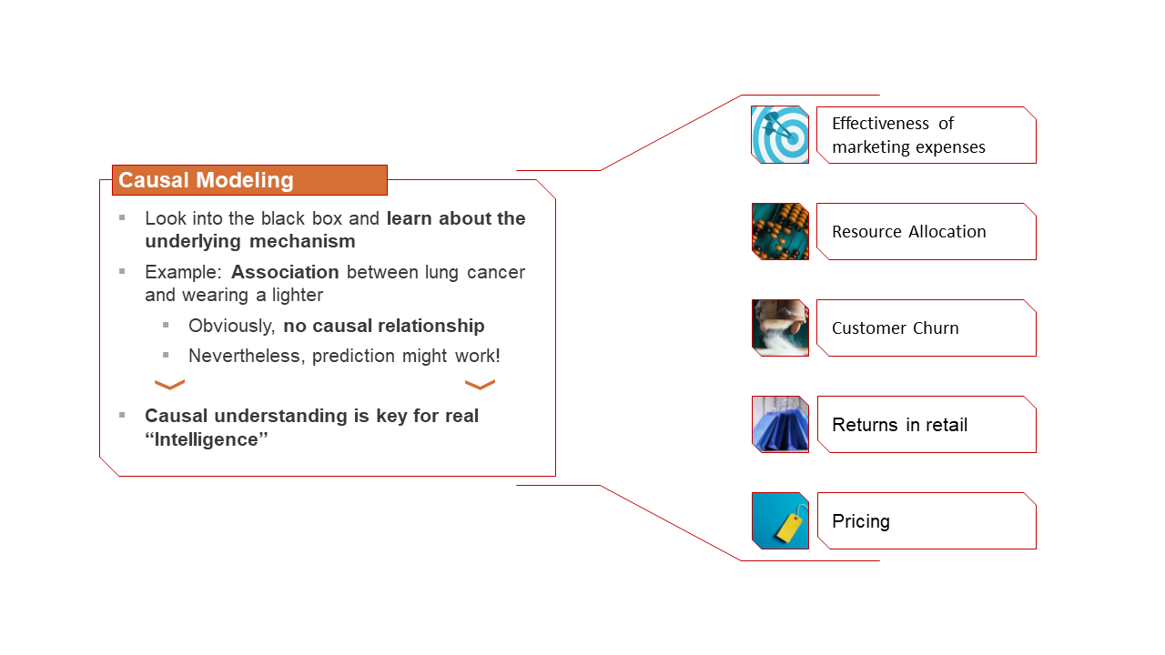
Causal Modelling

What is the causal effect of a treatment \(A\) on an outcome \(Y\)?

“Why do customer churn?”

“How can we retain customers?”

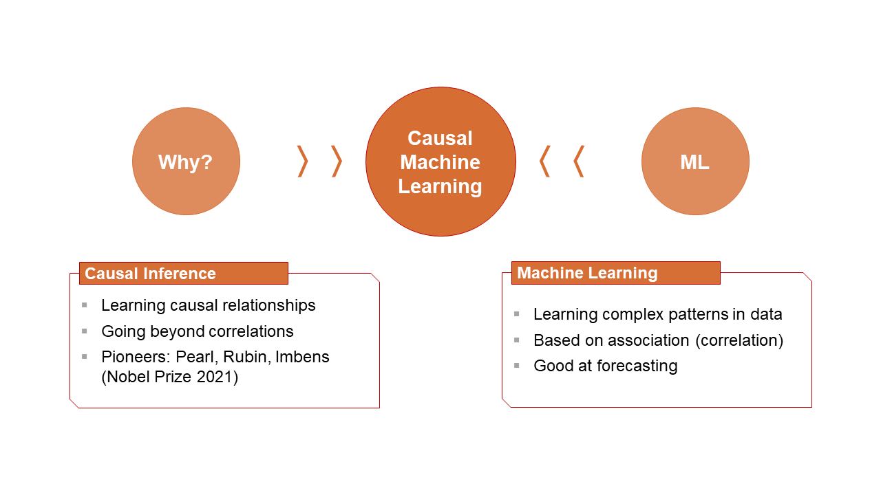
Causal ML: How can we use state-of-the art ML methods for causal inference?

Causal Inference: A Brief Introduction

Introduction to Causal Inference

How to assess causality with data?

• Approach

  1. Define causal parameters of interest
  2. State necessary assumptions for identification and valid estimation

• Helpful tools in causal inference

  • Potential Outcomes (PO) framework
  • Directed Acyclic Graphs (DAGs)

• General question

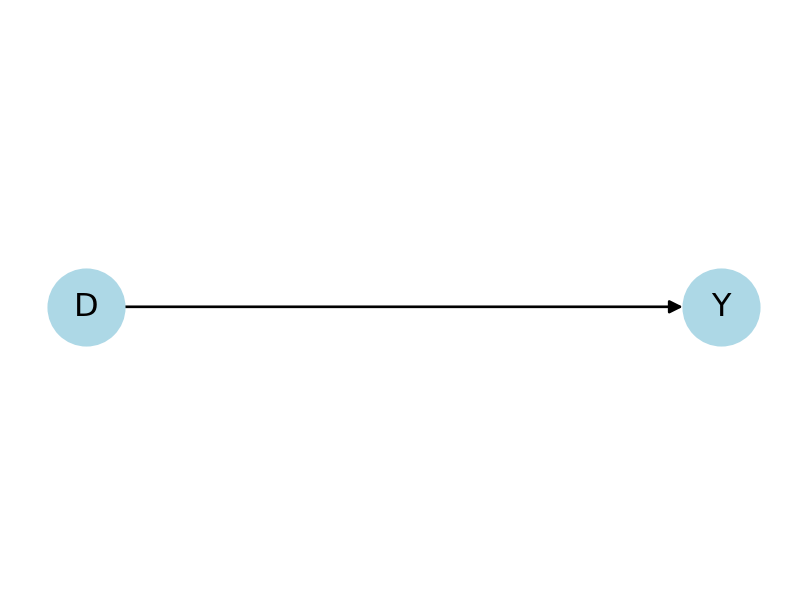
  What is the causal effect of treatment \(D\) on outcome \(Y\)?

Introduction to Causal Inference

Example: Uplift Modeling

Key questions:

1. What is the causal effect of an email campaign (coupon) (\(=D\)) on product sales (conversion) (\(=Y\))?

2. How to optimally target coupons (\(=D\)) towards newsletter subscribers?

Definition: Causal Effects

• Binary treatment \(D\) \[\begin{equation}D = \begin{cases}1, & \text{if treated ( = with coupon)}\\ 0, & \text{if not treated ( = without coupon)}\end{cases}\end{equation}\]

Potential outcome framework

• Define the potential outcomes as

  • \(Y(1)\): Conversion if she would receive a discount

  • \(Y(0)\): Conversion if she would not receive a discount

• Individual causal effect (ICE) \[\Delta = Y(1) - Y(0).\]

• Reference: Huber (2023)

Graphical Representation

Directed Acyclic Graphs (DAGs)

• DAGs help to communicate/discuss causal problems

• DAGs can be used to assess statistical dependencies between variables ( \(d\)-separation)

• Some of these statistical relationships might sometimes be unexpected (bad controls)

• References: Glymour, Pearl, and Jewell (2016), Cinelli, Forney, and Pearl (2022)

Code

import networkx as nx
import matplotlib.pyplot as plt

G = nx.DiGraph()

# Add nodes
G.add_node("D")
G.add_node("Y")
G.add_edge("D", "Y")

# Draw the graph
plt.figure(figsize=(4, 3)) 
pos = {"D": (0, 0), "Y": (2, 0)}
nx.draw(G, pos, with_labels=True, node_size=800, node_color='lightblue')
plt.show()

DAG: Causal Effect of D on Y.

Fundamental Problem of Causal Inference

Individual causal effects cannot be identified, in general.

• We only observe one of the potential outcomes \(\Rightarrow\) Factual

• The other outcome is unobserved \(\Rightarrow\) Counterfactual

What can we do about this?

• Make assumptions, e.g., SUTVA assumption

• Use data and estimate causal parameters

Example/Question:

What would you do to estimate the causal effect of the coupon on the conversion rate?

Estimation of Causal Effects

• A/B test, Randomized Control Trial (RCT), experiment

Gold standard: Experiment, RCT, A/B test

Under certain assumptions, we can consistently estimate the Average Treatment Effect (ATE)¹ of treatment \(D\) on outcome \(Y\) \[ATE= E[Y(1)] - E[Y(0)].\]

Basic idea:

• Use sample-based estimates \(E[Y|d = 1]\) and \(E[Y|d=0]\) for \(E[Y(1)]\) and \(E[Y(0)]\), respectively

1. We use the ATE as the leading example in this lecture, but there are also other causal quantities of interest that can be identified under similar assumptions, e.g., the ATE for the Treated.

Estimation of Causal Effects

Why does it work?

In an RCT, the allocation of the treatment to individuals is assigned randomly

\(\Rightarrow\) Treatment assignment is independent of potential outcomes

• Individuals do not self-select into the treatment, i.e., they cannot pick that value of the treatment that is best for them (in terms of their potential outcomes)

Estimation of the ATE based on Data

How to estimate the ATE using data?

1. Run a two-sample \(t\)-test, or,

2. Use linear regression \[\begin{equation}E[Y|D] = \underbrace{\alpha}_{ \leadsto E[Y|D=0]} + \underbrace {\beta}_{\leadsto ATE} \cdot D\end{equation}.\]

Estimation of the ATE with Covariates

• Why account for covariates/individual characteristics \(X\) in an RCT?

• Uplift example: Individual characteristics, gender, shopping history \(\ldots\)

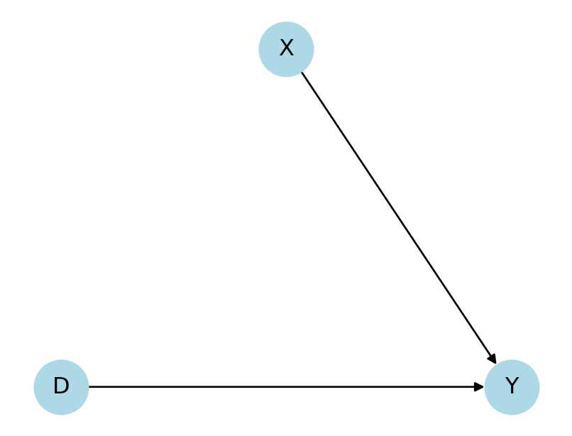
• Accounting for \(X\) s that help to explain \(Y\) can reduce the unexplained variation (increase power / efficiency).

• Randomization has to hold with respect to the covariates as well
  \(\Rightarrow\) Pre-treatment covariates

• Scope for more sophisticated evaluation: Conditional Average Treatment Effect (CATE) \(\Rightarrow\) Heterogeneity/Personalization \(\ldots\)

Estimation of the ATE with Covariates

Code

import networkx as nx
import matplotlib.pyplot as plt

G = nx.DiGraph()

# Add nodes
G.add_node("D")
G.add_node("Y")
G.add_node("X")
G.add_edge("D", "Y")
G.add_edge("X", "Y")

# Draw the graph
plt.figure(figsize=(4, 3)) 
pos = {"D": (0, 0), "Y": (2, 0), "X": (1,1)}
nx.draw(G, pos, with_labels=True, node_size=800, node_color='lightblue')
plt.show()

DAG: Causal Effect of D on Y, with predictive covariates X.

Estimation of the ATE with Covariates

Estimation with linear regression¹

\[\begin{align*}E[Y|D,X] = \underbrace{\alpha}_{ \leadsto E[Y|D=0]} + \underbrace{\beta}_{\leadsto ATE} \cdot D + \gamma X. \end{align*} \]

1. Disclaimer: Linear regression is only consistent under additional functional form assumptions such as linearity/homogeneity of ATE.

Estimation of Causal Effects … without Experiments?

• In an RCT, we can credibly justify that individuals do not self-select into the treatment status.

• But, what if an RCT is not feasible/available?

  • Examples: Randomization too costly (e.g., credit lines) or infeasible (e.g., removing standard services, enforcing memberships not possible)

  • Observational studies

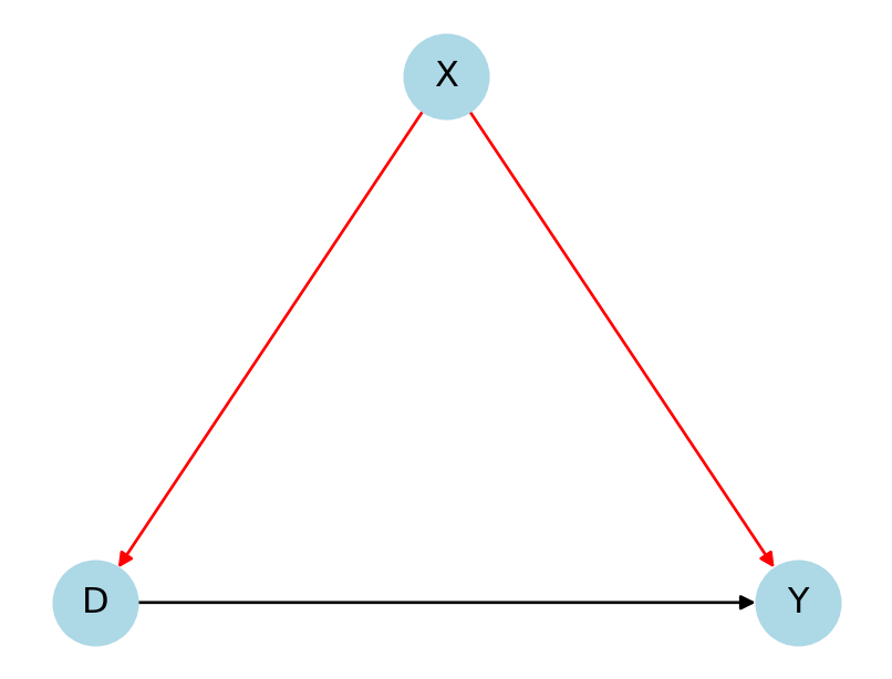
  • The treatment assignment might be confounded by observable variables \(X\) and unobservable variables \(U\) \(\Rightarrow\) The independence assumption might be violated.

Source: Facure and Germano (2021), Chapter 2.

Estimation of Causal Effects … without Experiments?

Code

import networkx as nx
import matplotlib.pyplot as plt

G = nx.DiGraph()

# Add nodes
G.add_node("D")
G.add_node("Y")
G.add_node("X")
G.add_edge("D", "Y")
G.add_edge("X", "Y")
G.add_edge("X", "D")

# Draw the graph
plt.figure(figsize=(4, 3)) 
pos = {"D": (0, 0), "Y": (2, 0), "X": (1,1)}
edge_colors = ['black', 'red', 'red']
nx.draw(G, pos, with_labels=True, node_size=800, node_color='lightblue',
 edge_color=edge_colors)
plt.show()

DAG: Causal Effect of D on Y, with confounders X.

Uplift Example (continued)

Experimental data

• Randomize the treatment \(D\) (coupon) to newsletter subscribers

• Independence assumption is satisfied

Observational data

• Use historic sales data

• Observe who has been treated (i.e., who used an email coupon) and who has not

• Account for confounding variables \(X\), e.g., shopping history

• Conditional independence is assumed

Challenges to Observational Studies

• If we can control for all confounding variables \(X\), the treatment is as good as randomly assigned conditional on \(X\) \(\Rightarrow\) We can estimate the \(ATE\)

  • Intuition: Matching on observables

• Assumption: Unconfoundedness/Selection on observables

  • Assumption (I): Independence of PO and treatment conditional on \(X\)’s

  • Assumption (II): Common support/overlap

  • (+ Assumptions that depend on the specific estimation framework used)

Estimation of the ATE with Confounders

• Estimation based on linear regression with covariates \(X\)

\[ \begin{equation}E[Y|D,X] = \underbrace{\alpha}_{ \leadsto E[Y|D=0]} + \underbrace{\beta}_{\leadsto ATE} \cdot D + \gamma X\end{equation}. \]

• \(\alpha = E[Y|D=0]\), \(\beta = ATE\)

• There are alternative estimation approaches available (imposing different assumptions)

  • Matching on observables / estimation in subgroups
  • Propensity score matching
  • Inverse probability weighting / standardization
  • Doubly robust approach / AIPW
  • Causal/Double Machine learning

So should we simply include all variables in the data?

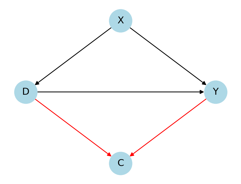
• Be careful! Don’t include bad controls/colliders.

• Collider bias/selection bias \(\Rightarrow\) Biases and spurious correlations

• Post-treatment covariates

• Model specification based on domain-specific expertise

Code

import networkx as nx
import matplotlib.pyplot as plt

G = nx.DiGraph()

# Add nodes
G.add_node("D")
G.add_node("Y")
G.add_node("X")
G.add_node("C")
G.add_edge("D", "Y")
G.add_edge("X", "Y")
G.add_edge("X", "D")
G.add_edge("D", "C")
G.add_edge("Y", "C")

# Draw the graph
plt.figure(figsize=(4, 3)) 
pos = {"D": (0, 0), "Y": (2, 0), "X": (1,1), "C": (1, -1)}
edge_colors = ['black', 'red', 'red', 'black', 'black']
nx.draw(G, pos, with_labels=True, node_size=800, node_color='lightblue',
 edge_color=edge_colors)
plt.show()

DAG: Causal Effect of D on Y, with confounders X and collider C.

Introduction to Double Machine Learning

Introduction to Double Machine Learning

Why ML for causal analysis?

• Machine Learning (ML) algorithms are powerful tools for predictions

• Use Case continued: Uplift modeling

  • Experiment, A/B test: Improve precision/efficiency/power
  • Account for confounding in observational studies
  • High-dimensional vector of covariates or complex relationship of \(Y\), \(D\) and \(X\).

Introduction to Double Machine Learning

Why ML for causal analysis?

Introduction to Double Machine Learning

Double Machine Learning (DML) approach (Chernozhukov et al. 2018)

• General framework for ML-based inference on a causal parameter, \(\theta_0\), for example, \[ \theta_0 = ATE = E[Y(1) - Y(0)] \]

• Use Case: With DML, we can estimate the ATE by using ML learners, such as gradient boosting, random forests, \(\ldots\)

• First, we need a formal causal model and a definition of the causal quantity of interest (=ATE)

Interactive Regression Model (IRM)

\[ \begin{align}\begin{aligned}Y = g_0(D, X) + U, & &\mathbb{E}(U | X, D) = 0,%\\D = m_0(X) + V, & &\mathbb{E}(V | X) = 0, \end{aligned}\end{align} \]

with the ATE being

\[ \theta_0 = \mathbb{E}[g_0(1, X) - g_0(0,X)]. \]

Here, \(\mathbb{E}[g_0(1, X)]\) and \(\mathbb{E}[g_0(0,X)]\) denote the expected value of the outcome variable with treatment status \(D=1\) and \(D=0\), respectively.

Interactive Regression Model (IRM)

Why ML for causal analysis?

\[ \begin{align}\begin{aligned}Y = \underbrace{g_0(D, X)}_{\text{ML Learner}} + U, & &\mathbb{E}(U | X, D) = 0.%\\D = m_0(X) + V, & &\mathbb{E}(V | X) = 0, \end{aligned}\end{align} \]

• In this model, we want to use flexible ML methods to estimate \(g_0(D, X)\) and in order to
  • Abstract from potentially restrictive assumptions, such as linearity or additivity
  • Model heterogeneous treatment effects using nonlinear learners
  • Handle high-dimensional data in terms of \(X\)

Introduction to Double Machine Learning

Why Double Machine Learning?

\[ \begin{align}\begin{aligned}Y = \underbrace{g_0(D, X)}_{\text{ML Learner}} + U, & &\mathbb{E}(U | X, D) = 0.%\\D = m_0(X) + V, & &\mathbb{E}(V | X) = 0, \end{aligned}\end{align} \]

• Why not simply estimate \(g_0(D,X)\) with ML and plug in predictions \(\hat{g}_0(D,X)\)?

• ML methods address the variance-bias-tradeoff by introducing some kind of regularization

• This will translate into a bias of the causal estimate

Uplift modeling example: Interactive Regression Model (IRM)

Challenges in causal machine learning

• Causal estimation after using ML methods for estimation require adjustments of the estimation framework \(\Rightarrow\) Chernozhukov et al. (2018)

The Key Ingredients of DML

1. Neyman orthogonality

2. High-quality ML estimation

3. Sample splitting

Neyman Orthogonality: Motivation

• We want to make estimation of the ATE robust against the regularization bias of ML learners

• This can be achieved by using an orthogonal estimation framework

• Neyman orthogonality states that the error terms that arise due to regularization do not affect the causal estimate

Neyman Orthogonality: Formal Definition

Technically, the inference framework is built on a moment condition that satisfies the property of Neyman orthogonality, i.e.,

\[\mathbb{E}[\underbrace{\psi(W; \theta_0, \eta_0)}_{\text{score function}}] = 0,\] with \(W\) denoting the data, \(\theta_0\) the causal parameter of interest (ATE), and \(\eta\) the nuisance part.

Neyman orthogonality ensures that the moment condition identifying \(\theta_0\) is insensitive to small pertubations of the nuisance function \(\eta\) around \(\eta_0\)

\[\left.\partial_\eta \mathbb{E}[\psi(W; \theta_0, \eta)] \right|_{\eta=\eta_0} = 0.\]

Neyman Orthogonality: IRM Example

Plug-in approach (not orthogonal)

\[\begin{align} \psi (W, \theta_0, \eta) = & g_0(1, X) - g(0,X) - \theta_0, \end{align}\]

with the nuisance parameter being

\[\begin{align} \eta &= (g(1, X), g(0,X)), \\ \eta_0 &= (g_0(1, X), g_0(0,X)) \end{align}\]

Neyman Orthogonality: IRM Example

Neyman-orthogonal score (doubly robust score)

\[ \begin{align} \psi (W, \theta_0, \eta_0) = & g(1,X) - g(0,X) \\ & + \frac{D (Y - g(1,X))}{m(X)} - \frac{(1 - D)(Y - g(0,X))}{1 - m(x)} \\ & - \theta, \end{align} \]

with the nuisance parameter

\[ \begin{align} \eta &= (g(1, X), g(0, X), m(X)), \\ \eta_0 &= (g_0(1, X), g_0(0, X), m_0(X)), \end{align} \]

with the propensity score \(m_0 = \mathbf{P}(D = 1 | X)\) which we have to estimate in order to achieve orthogonality, see DoubleML User Guide for more details.

Neyman Orthogonality: Use Case Example

• Non-orthogonal score in uplift example

def dml_score_nonorth(y, d, g_hat0, g_hat1, m_hat, smpls):

  # g_hat1, g_hat0 are the outcome predictions under treatment and control, respectively
  psi_b = g_hat1 - g_hat0

  # m_hat is the internally estimated propensity score
  psi_a = np.full_like(m_hat, -1.0)

  return psi_a, psi_b

from lightgbm import LGBMClassifier
ml_g_boost = LGBMClassifier(n_estimators=1000, learning_rate=0.005)
ml_m_boost = LGBMClassifier(n_estimators=1000, learning_rate=0.005)

np.random.seed(3141)
dml_obj_nonorth = dml.DoubleMLIRM(obj_dml_data=dml_data,
                                 ml_g=clone(ml_g_boost),
                                 ml_m=clone(ml_m_boost),
                                 n_folds=2,
                                 n_rep=1,
                                 trimming_threshold=0.01,
                                 score=dml_score_nonorth)
dml_obj_nonorth.fit()

Neyman Orthogonality: Use Case Example

• Comparison of non-orthogonal score to orthogonal score

Orthogonality: How Does it Work?

• The plug-in approach allows for valid estimation of the ATE, \(\theta_0\), whenever we can precisely estimate \(g_0(1,X)\) and \(g_0(0,X)\)

• Example: \(g_0(1,X)\) and \(g_0(1,X)\) are simply linear functions of the covariates \(X_1\) and \(X_2\) and the causal effect is constant and additive, such that

\[ \begin{align} g_0(1,X) &= \alpha + \theta_0 + \gamma_1 X_1 + \gamma_2 X_2,\\ g_0(0,X) &= \alpha + \gamma_1 X_1 + \gamma_2 X_2. \end{align} \]

• Then we could estimate \(\theta_0\) by simply using a correctly specified linear regression model

• However, this would not necessarily work if we used Lasso. Can you see why?

Orthogonality: How Does it Work?

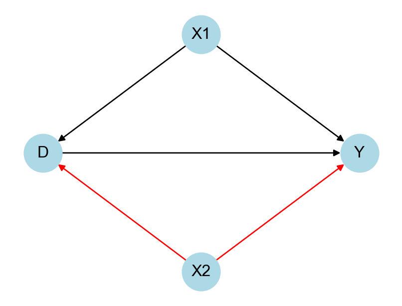
• The \(\ell 1\)-penalization of Lasso would reduce some of the coefficients in \(\gamma = (\gamma_1, \gamma_2)\) towards zero and maybe set some of them exactly to zero, say \(\gamma_2\) for the confounder \(X_2\)

• This is equivalent to removing the confounder \(X_2\) from the causal model
  \(\Rightarrow\) Ommited variable bias / confounding bias

Code

import networkx as nx
import matplotlib.pyplot as plt

G = nx.DiGraph()

# Add nodes
G.add_node("D")
G.add_node("Y")
G.add_node("X1")
G.add_node("X2")
G.add_edge("D", "Y")
G.add_edge("X1", "Y")
G.add_edge("X1", "D")
G.add_edge("X2", "D")
G.add_edge("X2", "Y")

# Draw the graph
plt.figure(figsize=(4, 3)) 
pos = {"D": (0, 0), "Y": (2, 0), "X1": (1,1), "X2": (1, -1)}
edge_colors = ['black', 'black', 'black', 'red', 'red']
nx.draw(G, pos, with_labels=True, node_size=800, node_color='lightblue',
 edge_color=edge_colors)
plt.show()

DAG: Causal Effect of D on Y, with confounders \(X_1\) and \(X_2\).

Orthogonality: How Does it Work?

• Using the orthogonal score makes estimation of the ATE robust against such estimation errors, if they are moderate

• In the IRM, this is done by including the propensity score in the orthogonal score \(\psi(\cdot)\)

• We can estimate \(\theta_0\) consistently, if the nuisance parameters \(g_0(1,X)\), \(g_0(0,X)\) and \(m_0(X)\) are estimated good enough

We will know see what good enough means…

High-Quality ML Estimation

• The nuisance parameters are estimated with high-quality (fast-enough converging) machine learning methods.

• Different structural assumptions on \(\eta_0\) lead to the use of different machine-learning tools for estimating \(\eta_0\) (Chernozhukov et al. 2018, sec. 3)

• Rate requirement in the IRM for estimation of ATE: \[\lVert \hat{m}_0 - m_0 \rVert_{P,2} \times \lVert \hat{\ell}_0 - \ell_0\rVert _{P,2} \le \delta_N N^{-1/2}\]

• \(\Rightarrow\) We can use ML methods, that have typically slower convergence rates than the parametric \(N^{1/2}\) (as for a correctly specified linear regression model)

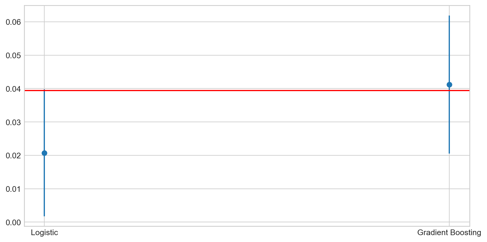
High-Quality ML Estimation: Use Case Example

• Comparison of the performance of the ML-based causal model to estimation based on (unpenalized) logistic regression

print(dml_obj_linear.evaluate_learners())
print(dml_obj_linear.evaluate_learners(metric=balanced_accuracy))

{'ml_g0': array([[0.45735802]]), 'ml_g1': array([[0.44600344]]), 'ml_m': array([[0.48082561]])}
{'ml_g0': array([[0.49937559]]), 'ml_g1': array([[0.51025686]]), 'ml_m': array([[0.6107002]])}

print(dml_obj_orth.evaluate_learners())
print(dml_obj_orth.evaluate_learners(metric=balanced_accuracy))

{'ml_g0': array([[0.46770032]]), 'ml_g1': array([[0.44701511]]), 'ml_m': array([[0.4792336]])}
{'ml_g0': array([[0.51123643]]), 'ml_g1': array([[0.53925407]]), 'ml_m': array([[0.61656226]])}

High-Quality ML Estimation: Use Case Example

• Comparison of the performance of the ML-based causal model to estimation based on (unpenalized) logistic regression

Sample-Splitting

• To avoid the biases arising from overfitting, a form of sample splitting is used at the stage of producing the estimator of the main parameter \(\theta_0\).

• Informal example:

  • Split data 50/50 into train (T1) and test (T2) samples
  • Fit ML algorithms on T1
  • Generate predictions for the T2
  • Plug predictions into score function and solve for \(\theta\)
  • Apply DML results to obtain confidence intervals, standard errors and \(p\)-values

• Efficiency gains by using cross-fitting (swapping roles of samples for train / hold-out)

Sample-Splitting

• To avoid the biases arising from overfitting, a form of sample splitting is used at the stage of producing the estimator of the main parameter \(\theta_0\).

• Informal example:

  • Split data 50/50 into train (T1) and test (T2) samples
  • Fit ML algorithms on T2
  • Generate predictions for the T1
  • Plug predictions into score function and solve for \(\theta\)
  • Apply DML results to obtain confidence intervals, standard errors and \(p\)-values

Sample-Splitting

Visualization of the DML (2) Algorithm

High-Quality ML Estimation: Use Case Example

• Comparison of estimation without sample-splitting to simple train-test-split and cross-fitting (all models with orthogonal score)

np.random.seed(3141)
dml_obj_no_split = dml.DoubleMLIRM(obj_dml_data=dml_data,
                             ml_g=clone(ml_g_boost),
                             ml_m=clone(ml_m_boost),
                             n_folds=1,
                             n_rep=1,
                             trimming_threshold=0.01,
                             apply_cross_fitting=False)

dml_obj_no_split.fit()

High-Quality ML Estimation: Use Case Example

• Comparison of estimation without sample-splitting and cross-fitting (all models with orthogonal score)

Main Result: Double Machine Learning

Main result in Chernozhukov et al. (2018)

There exist regularity conditions, such that the DML estimator \(\tilde{\theta}_0\) concentrates in a \(1/\sqrt{N}\)-neighborhood of \(\theta_0\) and the sampling error is approximately \[\sqrt{N}(\tilde{\theta}_0 - \theta_0) \sim N(0, \sigma^2),\] with \[\begin{align}\begin{aligned}\sigma^2 := J_0^{-2} \mathbb{E}(\psi^2(W; \theta_0, \eta_0)),\\J_0 = \mathbb{E}(\psi_a(W; \eta_0)).\end{aligned}\end{align}\]

Examples

You can play around with the three key ingredients in this

🦏 Shiny App 🦏

References

References

Bach, Philipp, Victor Chernozhukov, Malte S Kurz, and Martin Spindler. 2022. “DoubleML-an Object-Oriented Implementation of Double Machine Learning in Python.” Journal of Machine Learning Research 23: 53–51.

Bach, Philipp, Victor Chernozhukov, Malte S Kurz, Martin Spindler, and Sven Klaassen. 2021. “DoubleML – An Object-Oriented Implementation of Double Machine Learning in R.” https://arxiv.org/abs/2103.09603.

Chernozhukov, Victor, Denis Chetverikov, Mert Demirer, Esther Duflo, Christian Hansen, Whitney Newey, and James Robins. 2018. “Double/Debiased Machine Learning for Treatment and Structural Parameters.” The Econometrics Journal 21 (1): C1–68. https://onlinelibrary.wiley.com/doi/abs/10.1111/ectj.12097.

Chernozhukov, Victor, Christian Hansen, Nathan Kallus, Martin Spindler, and Vasilis Syrgkanis. forthcoming. Applied Causal Inference Powered by ML and AI. online.

Cinelli, Carlos, Andrew Forney, and Judea Pearl. 2022. “A Crash Course in Good and Bad Controls.” Sociological Methods & Research, 00491241221099552.

Facure, Matheus, and Michell Germano. 2021. “matheusfacure/python-causality-handbook: First Edition.” Zenodo. https://doi.org/10.5281/zenodo.4445778.

Glymour, Madelyn, Judea Pearl, and Nicholas P Jewell. 2016. Causal Inference in Statistics: A Primer. John Wiley & Sons.

Huber, Martin. 2023. Causal Analysis: Impact Evaluation and Causal Machine Learning with Applications in r. MIT Press.